Centre d'apprentissage

More on Sparse PCE Methods

---

Continuing the discussion on Polynomial Chaos Expansion (PCE) surrogate models from previously in Part 8, we will now cover the different settings for PCE surrogate model creation, including how to control the accuracy of the PCE representation.

Polynomial Chaos Expansion in Several Variables

PCE surrogate models can be constructed for any number of variables or input parameters. For a surrogate model with multiple quantities of interest, each quantity will have its own PCE surrogate model function. Therefore, it suffices to focus on a single output parameter while considering multiple input parameters:

The function is typically represented by a finite element model or other numerical method and we would like to approximate it with a PCE surrogate model. To do so, assume that the input parameters h ave certain probability distributions. We introduce random variables that represent the stochastic properties of . We can represent the function as:

where are orthogonal polynomials associated with the probability distributions of the random variables , and are the coefficients to be determined.

This notation is a bit cumbersome, so instead a multi-index notation can be used for the infinite expansion:

For a truncated expansion we get:

where and and is the maximum total polynomial degree that we would like to include.

The total degree of a multi-index is defined as:

For example, consider the following polynomial:

The term has a multi-index of and a total degree of ; the term has a multi-index of and a total degree of ; and the term has a multi-index of and a total degree of .

This can be generalized to products of different orthogonal polynomials by considering the highest degree for each polynomial. For example, using the analytical case covered in More on PCE Surrogate Models in Two Variables, where we considered an expansion with Legendre and Hermite polynomials in two variables, the term has a multi-index of . The total degree of this term is then . Note that the individual orthogonal polynomials have a range of lower monomial degrees when considered as general polynomials. For example, the term: has multi-index , in this context, reflecting the highest degree term only.

Instead of constructing a PCE representation for all polynomials up to a certain total degree , a more efficient representation is made possible by instead truncating the expansion based on the q-norm, which is formally only a quasi-norm and defined as:

for taking real values between and . Note that for , we get the standard total degree norm.

Using a q-norm condition, , for emphasizes the main effects and lower-order interactions, which are often more significant in practice. Typically, only a few lower-order terms are significant, while higher-order interactions can often be neglected. For example, truncating the expansion by using the q-quasi-norm for and , higher-order interaction terms like are excluded while terms like are included. Interaction terms in PCE are those with at least two indices greater than zero.

Note that although the input variables are assumed to be independent, there can still be interaction terms. These interaction terms represent the combined effect of two or more input variables on the quantity of interest (output). They capture how the response changes when multiple inputs vary simultaneously, beyond the sum of their individual effects, in a nonadditive way. For instance, a response surface could be curved such that the effect of changing depends on the level of , indicating an interaction.

The following calculations show which terms are included in the case with :

For the case with Legendre and Hermite polynomials, the resulting PCE approximation will then be:

This can be illustrated by plotting the multi-index of the included terms as points in a 2D plot, as shown below.

Multi-index plot for the included terms using and a maximum total degree of .

The following table with plots shows multi-indices for included terms for a few different q-norm values and a total degree less than or equal to . From these plots we can see that for we only get the main effect terms, the terms without interaction effects. For , we get a standard truncation based on total polynomial degree, including all interaction terms.

Multi-Index Plots for Various Quasi-Norm Values (q)
Included polynomial terms for , .	Included polynomial terms for ,.
Included polynomial terms for ,.	Included polynomial terms for ,.

The following figure shows the multi-index pattern for the PCE surrogate model default values with . The boundary of the included terms has a hyperbolic shape. An expansion based on this technique is referred to as a hyperbolic PC expansion.

The hyperbolic shape of the included polynomial terms in a PCE.

PCE Construction Methods

There are two methods available for creating a PCE surrogate model: Sparse Polynomial Chaos Expansion (SPCE) and Adaptive Sparse Polynomial Chaos Expansion (ASPCE). A sparse representation of PCE involves selecting a subset of polynomials from the full set of truncated polynomial expansions. By choosing only the most significant polynomial terms, this approach reduces the model's complexity while maintaining its accuracy and helps avoid overfitting. Note that the method of including polynomial terms based on the q-norm is only one contributor to the sparse subset selection. The other contributor is the least-angle regression (LARS) method, discussed below.

The SPCE and ASPCE methods offer several user-defined parameters that can enhance the accuracy of the approximation. Typically, increasing the number of input points (sampling points) is the primary option to consider for improving accuracy. Other parameters are generally considered advanced options and, in most cases, do not need to be adjusted.

Sparse Polynomial Chaos Expansion (SPCE)

The figure below shows the Uncertainty Quantification study settings with the Surrogate model option set to Sparse polynomial chaos expansion. This option has two user-defined settings: Relative tolerance (default 0.001) and Q norm, (default 0.5).

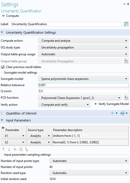
The settings for the Surrogate model option Sparse polynomial chaos expansion.

The SPCE method implements an adaptive algorithm based on a least-angle regression selection (LARS) method that iteratively selects the most significant terms in the truncated polynomial expansions. During the iterative process, the algorithm begins with the lowest possible polynomial order and gradually increases it, only adding new polynomial terms that are significantly correlated with the residual based on the already computed polynomial basis. During this process, the algorithm also ensures that the q-norm condition is met. The sparse representation is used both to reduce computational cost and to avoid overfitting. Note that a lower q-norm value can be used to further reduce the risk of overfitting.

The residual is computed by evaluating the PCE at the sample points. These sample points are selected using a Latin Hypercube Sampling (LHS) method. The number of sampling points is typically chosen automatically but can also be manually defined.

At the end of each LARS step, the SPCE method compares the leave-one-out cross-validation error to the Relative tolerance value. For both the SPCE and ASPCE methods, the truncated sparse coefficients are computed with an ordinary-least-square method in each adaptive step. This process continues until the error is smaller than the Relative tolerance value. If the maximum polynomial degree is reached without meeting the tolerance criterion, the surrogate model construction terminates. In this case, a warning is printed to the Log window, and a warning icon appears in the model tree under the Job Configurations > Uncertainty Quantification node, as shown below.

The warning indicator shows that the relative tolerance criterion was not met.

For the Compute action set to Compute and analyze, the default Automatic setting for the Number of input points is , where is the number of input parameters. For the Compute action set to Improve and analyze, the default value is . You can change this to a user-defined value by selecting Manual for the Number of input points type setting. This setting specifies the number of sample points used by the LHS algorithm. Increasing this number will typically enhance the approximation accuracy. However, a higher number also means more model evaluations, which can be time-consuming depending on the finite element model (or other numerical model) being approximated.

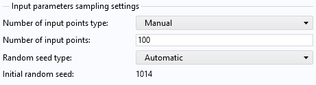
The Manual option for the Number of input points used for Latin hypercube sampling, here set to 100.

The value for the maximum total polynomial degree rarely needs to be changed due to the fact that the iterative process usually terminates before this number is reached. However, if needed, this value can be set at the Job Configurations level in the Settings window of the Job Configuration > Uncertainty Quantification node, as shown in the figure below. This setting is also available for the ASPCE method.

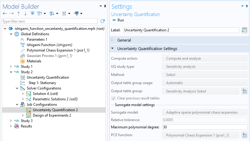
The Maximum polynomial degree setting, here shown with the default value .

In summary, to increase the accuracy of a PCE surrogate model using the SPCE method, you can lower the relative tolerance, adjust the q-norm, or increase the number of input points. Most commonly, increasing the number of input points will have the greatest impact on accuracy, though it is also the most computationally demanding option. If there are significant interactions in the model, increasing the q-norm may be necessary to capture these complexities effectively. However, this approach can also increase the risk of overfitting.

Adaptive Sparse Polynomial Chaos Expansion (ASPCE)

The figure below shows the Uncertainty Quantification study Settings window with the Surrogate model option set to Adaptive sparse polynomial chaos expansion. This option has one user-defined setting: Relative tolerance (default 0.001). It is the default method for Sensitivity analysis.

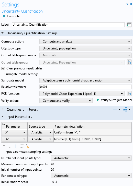
The Uncertainty Quantification study Settings window, which uses an ASPCE surrogate model.

Just like the SPCE method, the ASPCE method uses an adaptive algorithm based on the LARS method to select significant sparse coefficients from the truncated polynomial expansion. However, unlike SPCE, the ASPCE method adaptively learns the q-norm rather than requiring it to be user-defined, hence its name.

In the APCE method, the number of sampling points is not fixed. Instead, new sampling points are successively added using the LHS method, and a new error estimate is computed at each step.

Depending on whether the a posteriori cross-validation error estimation satisfies the relative tolerance, the method adds more input points selected by the LHS method. This allows for more model evaluations and the training of a new PCE at each adaptive step.

When the Compute action is set to Compute and analyze, the default Automatic setting for the Maximum number of input points is , where is the number of input parameters. The default setting for the Initial number of input points is . When the Compute action is set to Improve and analyze, the default values are and , respectively. You can change these values by selecting the Manual option. Just like for the SPCE method, increasing this number will typically enhance the approximation accuracy, but increase the computational cost.

Error Estimation

The error in the PCE approximation compared to the observed data is estimated using a version of the leave-one-out cross-validation (LOO-CV) method. The basic idea behind the LOO-CV method is to evaluate how well the PCE surrogate model predicts data points that were not used during its training. The LOO-CV method works by taking one data point out of the dataset, which will later be used for testing, while the remaining data points are used to train the model. The PCE model is then trained on the remaining data points. The left-out data point is used to test the model, and the prediction error is calculated and stored as the difference between the model's prediction and the actual value of the left-out point. This process is repeated for each data point in the dataset, with a different point being left out each time. After each data point has been left out once and tested, the average of the stored prediction errors is computed and used as the estimated total error.

The LOO-CV method has several benefits compared to more direct methods, such as a standard empirical training error computed by evaluating the least squares error at the training points. The least squares error tends to underestimate the true generalization error because it does not account for model performance on unseen data. Furthermore, the least squares error is sensitive to overfitting. A model with high complexity may fit the training data very well, resulting in a low least squares error, but may not generalize well to new data.

On the other hand, the LOO-CV method reduces sensitivity to overfitting because each prediction is made on a model trained on a slightly different dataset than the one used for evaluation. However, it is computationally more intensive than calculating the empirical error, as it requires retraining the model several times.

Further Learning

For more details on the LARS and LOO-CV methods, see G. Blatman, and B. Sudret, “Adaptive sparse polynomial chaos expansion based on least angle regression,” J. Comput. Phys., vol. 230, no. 6, pp. 2345–2367, 2011