Centre d'apprentissage

More on Covariance Functions

---

The theory of covariance functions is an important part of the definition of a Gaussian Process (GP) surrogate model. Here, we continue the discussion on GP surrogate models from Part 4 and give an introduction to the theory.

Covariance Functions

Similar to how the activation functions determine the characteristics of a deep neural network, the covariance functions determine the characteristics of a Gaussian process. We saw earlier how the squared exponential function generates smooth looking Gaussian processes. Let's now instead consider the exponential covariance function:

,

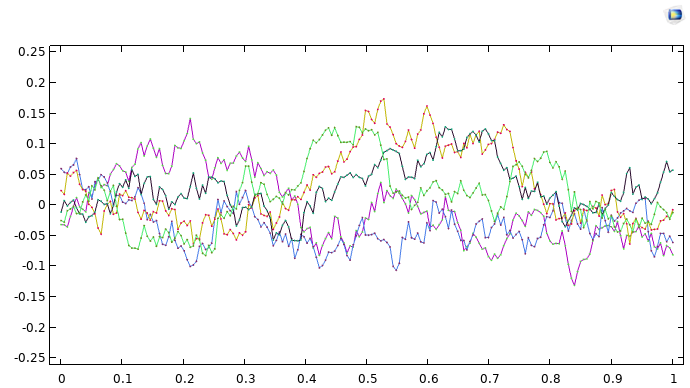
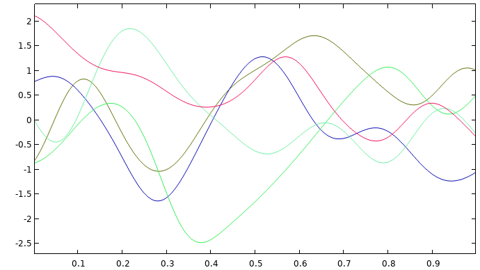
which generates a much rougher type of function. The figure below shows five sample functions drawn from a Gaussian process with an exponential covariance function.

This is not the greatest caption in the world. This is just a tribute.

Five Gaussian process functions on the unit interval with an exponential covariance function.

The function that the exponential covariance function generates is too rough to be used in surrogate models related to most physical phenomena. Instead, the squared exponential covariance function is more frequently used. However, the squared exponential covariance function can sometimes be too smooth, in which case a Matérn covariance function can be suitable. The Matérn covariance functions is a parametric family of functions that interpolates between the rougher exponential and the very smooth squared exponential covariance function. In general, a Matérn covariance function is parameterized by the variance ,  the correlation length , and an additional smoothness parameter .

In COMSOL Multiphysics^®, Matérn covariance functions for and are available. We can list some of the covariance functions in order of smoothness starting from the exponential covariance function, which is equivalent to the Matérn 1/2 covariance function, ending with the squared exponential covariance function, denoted . The squared exponential covariance function can be shown to correspond to the limit . Gaussian processes corresponding to are smoother than those for the exponential . Similarly, Gaussian processes corresponding to are smoother than those for , and so on. For random processes, standard notions of differentiability cannot be used. However, by using the concept of mean-square differentiability (see Further Learning resource on GP for machine learning), we can assign a level of differentiability to each Gaussian process. These properties are summarized in the following table.

Name		Covariance Function	Mean-square Differentiability	Available in COMSOL
Exponential			0	No
Matérn 3/2			1	Yes
Matérn 5/2			2	Yes
Squared Exponential				Yes

Half-integer Matérn covariance functions are preferred since they give much simpler covariance function expressions than whole integer ones, and this is why options for and are available in COMSOL^®. For and higher, the processes are hard to distinguish from the squared exponential, and therefore only the squared exponential option is included.

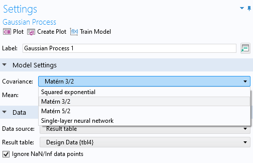
The figure below shows the Gaussian Process function Settings window with options for the different covariance functions. The default Covariance setting is Matérn 3/2.

The Gaussian Process function Settings window with the options for different covariance functions.

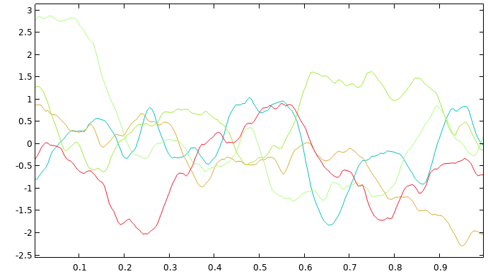
When performing Gaussian process regression, the choice of covariance function determines the level of smoothness of the fitted surrogate model function. This choice will also affect the fundamental assumption about the process that generated the underlying dataset and the pointwise standard deviation estimate. Selecting the appropriate covariance function is not always straightforward and is reminiscent of choosing an activation function for deep neural networks. Use any knowledge of the expected smoothness of the phenomena for which you are creating a surrogate model to choose a suitable level of smoothness. Note that, for practical purposes, the Matérn 3/2 and Matérn 5/2 covariance functions often produce quite similar surrogate models. Samples of GP functions based on these covariance functions are shown in the figures below (such sample functions are also referred to as sample paths).

A graph consisting of five different colored lines, each displaying a wave-like appearance.

Five GP functions on the unit interval for the Matérn 3/2 covariance function with zero mean.

A graph consisting of five different colored lines, each displaying a wave-like appearance.

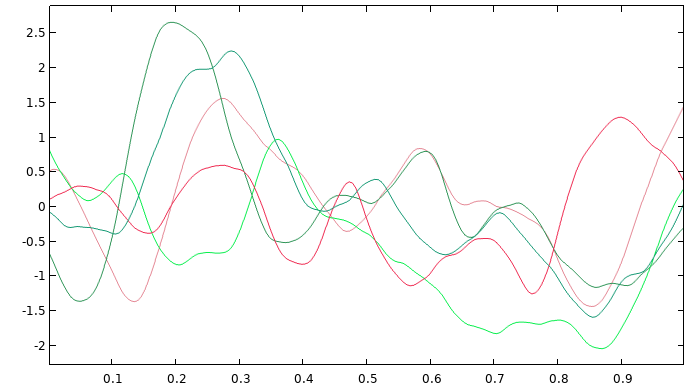
Five GP functions on the unit interval for the Matérn 5/2 covariance function with zero mean.

A graph consisting of five different colored lines, each displaying a wave-like appearance.

Five GP functions on the unit interval for the squared exponential covariance function with zero mean.

There is also a nonstationary covariance function option available, which is called the single-layer neural network kernel. This covariance function originates from the fact that there are theoretical links between DNN and GP models, and it can shown, for example, that important classes of neural network models become increasingly similar to GP models when the number of nodes in the neural network increases. For more information, see, for example, the resource on GP for machine learning under Further Learning, where this equivalence is demonstrated for a neural network with a single hidden layer.

Gaussian Processes as Sums of Covariance Basis Functions

The GP regression method, which GP surrogate models are based on, can also be seen as a systematic way of computing the weighted sum of covariance functions to approximate any continuous function arbitrarily well. This was explained briefly using the analogy to radial basis function (RBF) fitting in the course part detailing More on Gaussian Process Surrogate Models.

The expressions and plots below show a specific GP regression model based on three training points, using different covariance functions. Note that, unlike RBF fitting, GP regression does not necessarily need to interpolate the training data points, especially when the training data is noisy.

In this case, the Matérn functions do not interpolate exactly due to the fact that the same coefficients were used for all three cases. In a practical situation, the coefficients will change when switching covariance functions because the hyperparameters are optimized by the regression algorithm. This is explained in the next part detailing More on Hyperparameters for Gaussian Processes. In a real modeling situation, the number of terms can be several thousand since it equals the number of training data points. 

Squared Exponential Covariance Function Example

A plot of the weighted sum of three squared exponential covariance functions.

Matérn 5/2 Covariance Function Example

A plot of the weighted sum of three Matérn 5/2 covariance functions.

Matérn 3/2 Covariance Function Example

A plot of the weighted sum of three Matérn 3/2 covariance functions.

Although the mean square differentiability of the Matérn 3/2 and Matérn 5/2 processes are 1 and 2, respectively, the smoothness of the mean function, which corresponds to averaging over many sample functions, can be higher. In practical numerical implementations, when differentiating these functions using exact coefficients, term cancellations can occur. This can result in higher-than-expected differentiability: up to 2 for a Matérn 3/2 function and up to 4 for a Matérn 5/2 function. The squared exponential covariance function is infinitely differentiable.

Gaussian Processes in 2D and Higher Dimensions

Gaussian processes are applicable in any dimension. To see how the theory generalizes, we can look closer at the 2D case. Consider the squared exponential covariance function:

This expression generalizes to any dimension. We just need to replace the definition of distance with a 2D distance:

The structure of the covariance matrix for sampled points doesn't change when we move up in dimension and, for the 2D case, we can write each entry of the squared exponential covariance matrix as:

with

Notice that to sample a GP function in 2D in for instance, a 40-by-40 grid of points, we need the covariance between each of these 1600 points, which implies using a 1600-by-1600 sized covariance matrix. The higher the dimension, the more quickly we will run into the computational limitations of Gaussian processes.

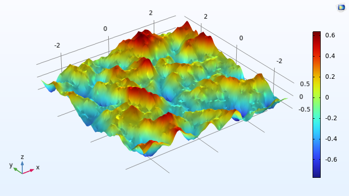
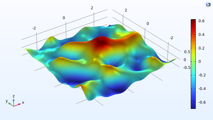
The figures below visualize realized 2D Gaussian processes for the Matérn 3/2, Matérn 5/2, and squared exponential covariance functions.

A plot in 3D space of a smooth, curving surface with several hills and valleys that has a rainbow color distribution.

A Gaussian process with the Matérn 3/2 covariance function with zero mean.

A plot in 3D space of a smooth, curving surface with several hills and valleys that has a rainbow color distribution.

A Gaussian process with the Matérn 5/2 covariance function with zero mean.

A plot in 3D space of a smooth, curving surface with multiple hills and valleys that has a rainbow color distribution.

A Gaussian process with the squared exponential covariance function with zero mean.

When creating surrogate models based on physics simulations, the input points may represent different physical quantities having different scales. In this case, different length scales are used for each input dimension. For two input variables, the expression for anisotropic length scale for the SE covariance is:

For higher dimensions, this becomes:

Further Learning

To learn more about Gaussian process regression, see the following references:

• Uncertainty Quantification Module User's Guide in the COMSOL Documentation
• C.K. Williams and C.E. Rasmussen, Gaussian processes for machine learning, MIT Press, Cambridge, MA, vol. 2, no. 3, p. 4, 2006.