Performing a Reliability Analysis UQ Study
To continue our analysis of the steel bracket model from Parts 2–4 of this course, here we perform a reliability analysis for the same input parameters used in Part 4. The Reliability Analysis UQ study type will enable us to estimate the probability that the misalignment angle exceeds a certain threshold — in this case, 0.1 degrees.
Reliability Analysis
From the uncertainty propagation analysis in Part 4, we learned from the QoI Confidence Interval table that the mean is about 0.09 degrees with a standard deviation of 0.003 degrees. The KDE plot, also obtained from the uncertainty propagation analysis, gives this information graphically, as shown in the figure below.

A KDE plot of the misalignment angle.
We can see that there appears to be some risk that the angle exceeds 0.1 degrees. To get a more accurate estimate of the risk for exceeding 0.1 degrees, we will run a reliability analysis. The reliability analysis will focus the model evaluations in the critical regions necessary to increase the accuracy of the surrogate model and thereby the requested probability estimate. Mathematically, we are asking for the probability  . In this example, achieving this probability value is the goal of the reliability analysis. We will use one condition to do this. In practice, however, a reliability analysis study can include multiple condition, as illustrated in the figure below. (The figure highlights a reliability analysis with multiple conditions and does not apply to our example.)

The contour lines for the two quantities of interest, q1 (blue) and q2 (purple), represent the thresholds q1 = 21 and q2 = 9.95, used in a particular reliability analysis (different from the steel bracket example of this article). In this illustration, two input parameters are plotted on the x- and y-axes. The shaded region indicates the range of input parameters that satisfy the reliability criteria, defined by q1 < 21 and q2 > 9.95.
Open the Model and Add the Study
For our example reliability analysis, we will build on the model from Part 4. Start by opening the model file for the UQ structural and uncertainty propagation analysis of a bracket. Save the file and rename it to bracket_uq_static_structural_and_reliability_analysis.mph.
Right-click Study 4 > Uncertainty Quantification and select Add New Uncertainty Quantification Study For Reliability Analysis, as shown in the figure below. The new study with the reliability analysis settings will be available as Study 5.
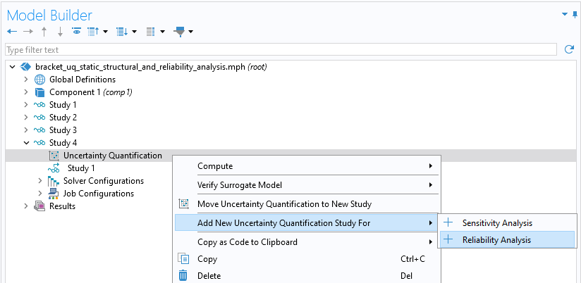 A screenshot of part of the model tree with the menu options for the Uncertainty Quantification study node expanded and the Reliability Analysis option selected.
Adding the UQ study type for reliability analysis.

Study 5 is the fourth Uncertainty Quantification study. This study has the reliability analysis option enabled.
In the Uncertainty Quantification node Settings window, the UQ study type is automatically set to Reliability analysis, EGRA. EGRA stands for efficient global reliability analysis and is discussed in more detail below. The settings for the Quantities of Interest and Input Parameters sections will automatically be copied over from the uncertainty propagation study, with the side length (ls) and cross-plate width (wp) as input parameters. The Quantities of Interest table now has additional columns for True if and Threshold.
For this example, type 0.1 for the threshold value. This corresponds to the condition  . (If you are working with the model version without fillets, note that the condition needs to be a bit higher,
  , in order to be meaningful.)
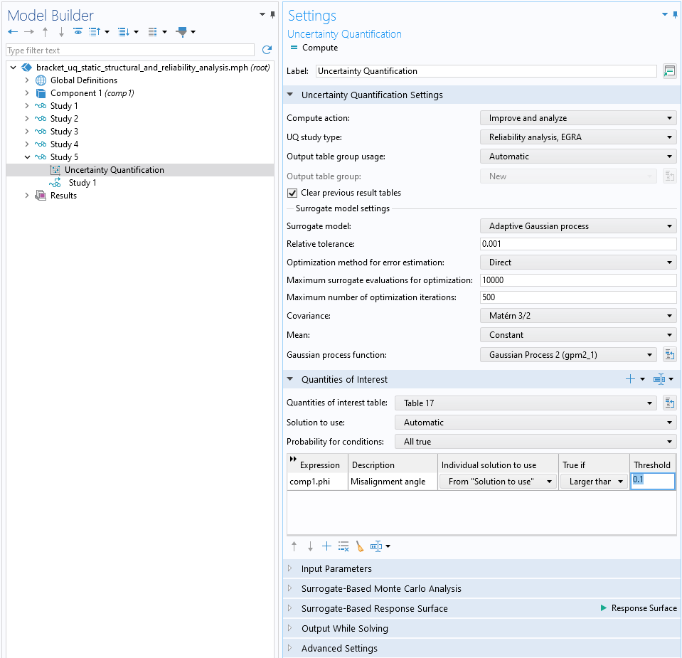 The Settings window for the reliability analysis with the Uncertainty Quantification Settings section and Quantities of Interest section expanded.
The reliability analysis settings in the Uncertainty Quantification node Settings window.
Like surrogate-based sensitivity analysis and uncertainty propagation, reliability analysis is also built using a surrogate model. It uses the EGRA method, which is based on an adaptive Gaussian Process (GP) surrogate model. This method strikes a balance between exploring regions where the GP model provides accurate predictions and focusing on areas where the GP has high variance and requires more model evaluations. The GP model does not need to achieve high accuracy in regions far from the limit state, where the quantities of interest (QoIs) are equal to the thresholds. This is accomplished by concentrating adaptive model evaluations around the limit state, the boundary regions defined by the threshold conditions, thereby reducing the overall number of model evaluations needed.
In this case, we will reuse parts of the analysis from the uncertainty propagation step by changing the Compute action setting selection to Improve and analyze.
Run the Simulation and Analyze the Results
To begin the reliability analysis computation, right-click Study 5 and select Compute. The computation takes about 5 minutes, depending on the hardware.
The result is available in the table under Reliability Analysis > Probability for Conditions, as shown in the figures below. Recall that we are calculating the probability that the angle will exceed 0.1 degrees. The table estimates this probability to be approximately 0.003, indicating a 0.3% risk that the misalignment angle will exceed 0.1 degrees under the given threshold condition.

The location of the Probability for Conditions table.

The Probability for Conditions table displaying the probability for the condition to be fulfilled.
Note that, for the version of the model without fillets, the probability for the alternative condition to be fulfilled is estimated to be approximately 0.02, or 2%.
Response Surface
The Uncertainty Quantification study includes an option for plotting a response surface where one of the quantities of interest is plotted against two of the input parameters. This is only available for those studies that uses a surrogate model. To plot a response surface, in the Uncertainty Quantification study settings, locate the Surrogate-Based Response Surface section and click the Response Surface button, as seen below. To get better resolution of the response surface, you can specify a larger distribution resolution for each input parameter.

The functionality for plotting response surfaces.
The response surface plot is a Table Surface plot with the label automatically changed to Response surface.

The location of the Response surface plot in the model tree.

The settings for the Table Surface plot used to plot a response surface.
In the Settings window for the Table Surface plot, you can change the pair of input parameters to consider, along with other settings. Note that clicking Create Plot in one of the surrogate models under Global Definitions provides similar functionality.
Uncertainty Propagation and Reliability Analysis for All Parameters
As mentioned earlier, some of the less significant parameters might still contribute notably to the uncertainty propagation and reliability analysis. To investigate this, we can include all of the parameters that were part of the screening and sensitivity analysis and run the uncertainty propagation and reliability analysis again. While this approach requires longer computation time, the results are provided here for completeness. The uncertainty propagation, including all parameters, takes about 45 minutes to complete, depending on hardware.

A KDE plot of the misalignment angle where all of the parameters are included in the analysis.
The QoI Confidence Interval table shows a mean of 0.09, which is consistent with the earlier analysis. The standard deviation is now about 0.004, which is slightly higher than the previous analysis, as expected, since varying additional input parameters gives a higher output variance.

The mean, standard deviation, minimum, maximum, and confidence interval values computed from the uncertainty propagation analysis where all parameters are included in the analysis.
The reliability analysis, when including all parameters, takes about 35 minutes to complete, depending on the hardware. In this case, the Probability for Conditions table shows that the probability of exceeding the 0.1 degree threshold is approximately 0.008, or 0.8%. This is significantly higher than the 0.3% estimate from the earlier simplified analysis, indicating that, despite the mean and standard deviation being comparable, including all parameters is crucial for an accurate reliability analysis in this case.

The Probability for Conditions table displaying the probability for the condition to be fulfilled.
Envoyer des commentaires sur cette page ou contacter le support ici.