Centre d'apprentissage

Introduction to Using Surrogate Models

---

The COMSOL^® software includes functionality for creating and using surrogate models. This functionality is available through:

• Specialized Surrogate Model Training and Uncertainty Quantification study types
• Design of experiments (DOE) methods
• Surrogate model function definitions

Using a surrogate model instead of a full-fledged finite element model as the basis of an app can greatly increase the app's computational speed. A surrogate model is usually more simple and computationally efficient than a finite element model and is used to approximate the behavior of models that are more complex and computationally expensive. Surrogate models evaluate models faster, providing app users with a more interactive experience, and enable an easier and wider adoption of simulation across organizations.

Surrogate models are also used in contexts beyond apps for any situation where reducing the computational requirements of a model, or part of a model, is needed. Uncertainty quantification is one such context, where the use of surrogate models enables statistical calculations that would otherwise not be feasible.

Here, we begin this course by explaining what a surrogate model is and how to create one with the software.

Understanding Surrogate Models

Before going into detail about the process of creating a surrogate model, let's look at the classical method of replacing a numerical model with a lookup table and using interpolation to estimate values. In COMSOL Multiphysics^®, lookup tables are commonly used to represent experimental data, which we will consider here as a form of surrogate model solely for illustration purposes. For example, the table below is used in the Temperature Field in a Cooling Flange tutorial model to represent the angular dependency of a heat transfer coefficient, as measured by experiments.

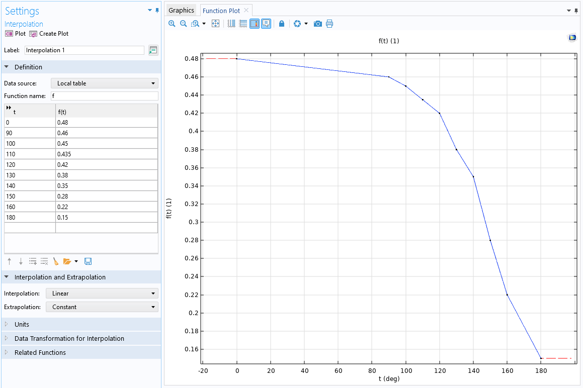The Settings window for the Interpolation function and the corresponding function plot of a line graph showing a blue line.

The Interpolation function used to define the angular dependency of a heat transfer coefficient.

To retrieve values in between the measured data points, you can choose between various interpolation methods: Nearest Neighbor, Linear, Piecewise cubic, or Cubic spline.

For the purpose of linear interpolation, you can also have tables representing two- or three-dimensional data. These tables can be entered directly into the user interface or loaded from a text file. An example of a text file can be seen in the image below: This image shows data for a material quantity called a transport number, which, in battery design simulation, is a function of concentration and temperature.

A text file containing the table data that defines the transport number for a battery model.

This data can be used to create a linear interpolation function in COMSOL Multiphysics^®. The table can then be visualized by creating a plot of the function, as pictured below.

The plot of the interpolation function used to define the transport number.

In two and three dimensions, the interpolation options are limited to nearest-neighbor or linear interpolation.

The table lookup method with linear interpolation can theoretically replace a numerical model and act as a surrogate model. However, this method does not perform well with models that have more than three input parameters and is not effective at capturing nonlinear or noisy behavior. Indeed, linear interpolation functions are only supported for up to three input parameters. In COMSOL Multiphysics^®, there are several methods for generating surrogate models that address these limitations. Like the table lookup method, these approaches use tabulated data, which can come from any type of output from a COMSOL model, other software, or experimental results. These are known as data-driven surrogate models and are nonintrusive, meaning they can be applied without altering the original numerical method used. Additionally, there are various reduced-order modeling methods based on different techniques.

In a way similar to that of representing material properties with an interpolation table, we can, in an abstract fashion, view a parametric COMSOL model as a function:

where are the input parameters, which could be length, width, material conductivity, coordinates, etc., and is some output quantity that we are interested in, such as temperature, mechanical stress, or electric current.

More generally, we can define multiple functions:

...

for all the output quantities, or quantities of interest, we are interested in.

In an app, a surrogate model function can be evaluated similarly to any other user-defined function. This allows the surrogate model function to replace the need for solving and evaluating the complete finite element solution (or solution based on other numerical methods). When evaluating a surrogate model function, you can generate the same types of visualizations as you would with a conventional solution, such as slice, surface, volume, streamline, and arrow plots.

In theory, one could consider performing a full parametric sweep over all input parameters to create a comprehensive and densely sampled dataset. However, this approach is often computationally prohibitive in many practical scenarios. Instead, the parameter space is usually sampled sparsely, and surrogate models are used to accurately approximate unsampled values. This need for sparse sampling is why DOE methods are frequently used in the data-generation step of creating data-driven surrogate models. These methods help to efficiently explore the parameter space and capture the essential variations needed for accurate model approximation.

Defining a Surrogate Model

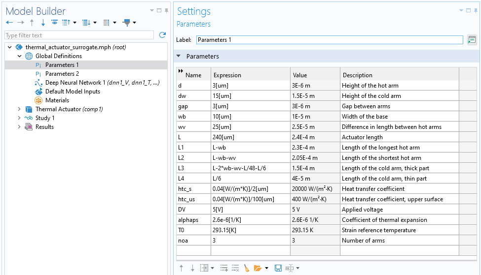
One way to create a surrogate model is to base a model on data from experimental results, such as material data. However, the typical starting point for creating a surrogate model is to build upon a COMSOL model driven by a set of parameters defined under Global Definitions. For instance, you could use the parameter set shown in the figure below, which is taken from the parameterized thermal actuator tutorial model.

The Model Builder with the Parameters 1 node selected and the corresponding Settings window, which contains a tabular list of parameters used in the model.

The parameters list for the parameterized thermal actuator tutorial model.

You can find a demonstration app based on this model in the software under the COMSOL Multiphysics section of the Application Libraries: COMSOL Multiphysics > Applications > tubular_reactor_surrogate. The model that this app is based on is extensively covered in the Learning Center course "Defining Multiphysics Models".

We might be interested in a version of this model where we can quickly evaluate the values of a set of output quantities based on certain ranges of input parameter values. Let's assume that we are interested in creating a surrogate model for predicting the variation in the maximum displacement of the tip of the actuator. Furthermore, assume that we vary just two of the model parameters, the actuator length and the applied voltage, according to the following table:

Parameter	Min Value	Max Value	Unit	Variable Name
Actuator length	150	400
Applied voltage	0.5	10

For the output quantity of interest, we have the maximum displacement.

Quantity of Interest	Type	Unit	Surrogate Model Function Name
Maximum displacement	Scalar

This defines a surrogate model function corresponding to one quantity of interest and two input parameters. Once we have identified the input parameters and output quantities of interest, we are ready to start creating a surrogate model. This will be discussed further later in the course, as well as how to expand the model to include additional input parameters and quantities of interest. Note that a surrogate model definition can have multiple quantities of interest, with one function defined for each.

The Surrogate Model Training Study

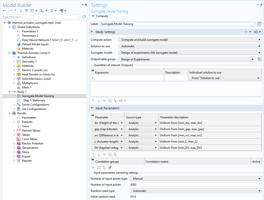
To create a surrogate model in COMSOL^®, you need to train a model on a dataset produced with the Surrogate Model Training study. It is recommended to train a surrogate model using strategic DOE sampling methods, such as Latin hypercube sampling (LHS), rather than conventional methods like random or uniform grid sampling. LHS is used in the Surrogate Model Training study and efficiently spans the input space without excessive amounts of data sampling. Although surrogate model accuracy improves when more data points are used, it is necessary to find a balance between the required model accuracy and the time it takes to generate more data points. The Surrogate Model Training study can be used for data generation that better achieves this balance. The study can also be used to enable automated surrogate model training following the data generation.

The Model Builder with the Surrogate Model Training study node selected and the corresponding Settings window.

The Surrogate Model Training study, used to generate the data required for training surrogate model functions.

Surrogate Model Functions

In COMSOL^®, you can find the surrogate models as functions under the Global Definitions node. Note that the different surrogate model options include their own specialized functionality as well as limitations, so it is essential that you select the surrogate model that best fits the requirements and constraints of the problem at hand. One of the surrogate models, Deep Neural Network (DNN), is included in COMSOL Multiphysics^®. The Uncertainty Quantification Module includes the Gaussian Process (GP) and Polynomial Chaos Expansion (PCE) surrogate models, as well as studies and analysis functionality that automatically employ the GP and PCE models.

If you are looking for a surrogate model that includes uncertainty estimates corresponding to the quality of data fitting, use the GP surrogate model; uncertainty estimates are not available in the DNN and PCE models.

The surrogate model functions are available under the Global Definitions node in the Model Builder.

Multidimensional Function Interpolation and Approximation

The surrogate models can be used for general multidimensional function interpolation and approximation and can handle an arbitrary number of inputs and outputs. The surrogate models are also well suited for handling complex nonlinear relationships in the data. Along with using surrogate model functions in apps and uncertainty quantification, they can be used to represent material data, for optimization, to replace parts of a multiphysics model, and more. The surrogate model functions can be differentiated multiple times with respect to any of the input parameters.

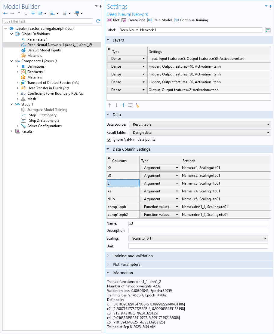The Model Builder with the Deep Neural Network function node selected and the corresponding Settings window.

The Settings window for a DNN surrogate model function.

The Surrogate Model Workflow

A typical workflow for creating and using a surrogate model is as follows:

1. Start with a full-fledged COMSOL Multiphysics model, which may be based on the finite element method or any of the other available numerical methods, such as the boundary element method, discontinuous Galerkin method, particle tracing, or ray optics.
2. Use the Surrogate Model Training study to generate Design Table data to be used for training the data-driven surrogate model. The Surrogate Model Training study employs design of experiments methods to efficiently sample the parameter space of the COMSOL Multiphysics model.
3. Choose a suitable surrogate model and train the model on the Design Table data.
4. Use the surrogate model to accelerate the computations of a model, an app, a digital twin, or system simulation.

Optionally, you can import tabulated experimental data to train a surrogate model in COMSOL Multiphysics.

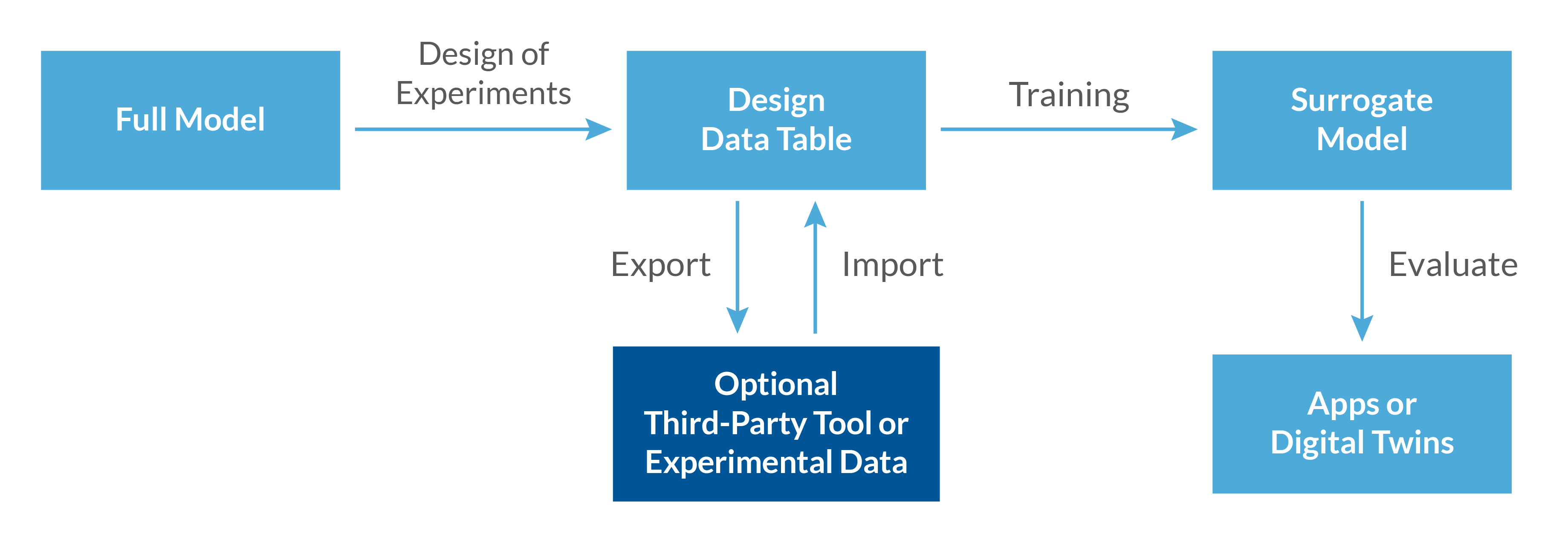A set of rectangles, each containing some text, with arrows pointing between them to indicate the general sequence of steps followed for creating and then using a surrogate model.

The workflow for creating and using a surrogate model.

In the following parts, we will learn about creating and using different types of surrogate models as well as how to generate training data using design of experiments.