
Have you ever had a set of nonuniformly distributed points in a Cartesian plane that sample a surface height, such as points on the contours of a map or data points representing some material property data? If so, you probably also wanted to reconstruct, or interpolate, a continuous and smooth surface between these points. You can construct such a surface using the core capabilities of COMSOL Multiphysics by using Radial Basis Functions. Let’s find out how…
An Introduction to Radial Basis Functions
A single Radial Basis Function (RBF) is any function defined in terms of distance (radius) from a point:
(1)
where is the weight of this RBF;
are the coordinates of the point, or center; and
is the distance from any other point in the xy-plane to this center.
The RBF itself can be one of many different types of functions. The family of polyharmonic splines is often used for interpolation, particularly the thin-plate spline function. The thin-plate spline basis function is:
(2)
Now, just a single one of these RBFs is not all that interesting, but we can take a sum over a finite number of different centers with different weights and optionally add a linear polynomial term with weights , giving us the function:
(3)
If there are enough centers, then this sum of a set of RBFs can be used to represent very complicated single-valued functions. When using the thin-plate spline basis, there is the added advantage that this function is also smooth everywhere and infinitely differentiable.
Let’s now take a look at how to interpolate a smooth surface with these RBFs. If we are given a finite set of center point locations, , and their corresponding known heights,
, then we can write a system of linear equations:
(4)
where the terms of the system matrix, , are the Radial Basis Functions evaluated between the centers.
Almost all of the off-diagonal terms will be nonzero when using the thin-plate spline basis, hence this system matrix is quite dense. The linear system can be solved for all of the weights and we can then evaluate the sum of our weighted RBFs at any other point in the xy-plane, giving us a smooth interpolation function. Let’s now look at how to compute these weights and visualize the interpolation function using the core capabilities of COMSOL Multiphysics.
Surface Interpolation with Radial Basis Functions in COMSOL Multiphysics
We start with a model containing a 3D component with a dimensionless units system. The units system is selected in the settings for Component 1. A dimensionless units system is simpler to use if our data represents material properties rather than a geometry.
The geometry in the model consists of two features. First, a Point feature is used to define the set of points. (The list of coordinates can be copied from a text file.) The Cumulative Selection is used to define a named selection of all of these points, as shown in the screenshot below. There is additionally a Block feature, which has dimensions that are slightly larger than the range of data points and is positioned to enclose all data points.
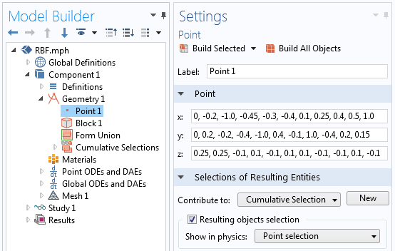
A screenshot showing the definition of the data points to interpolate and the cumulative selection definition.
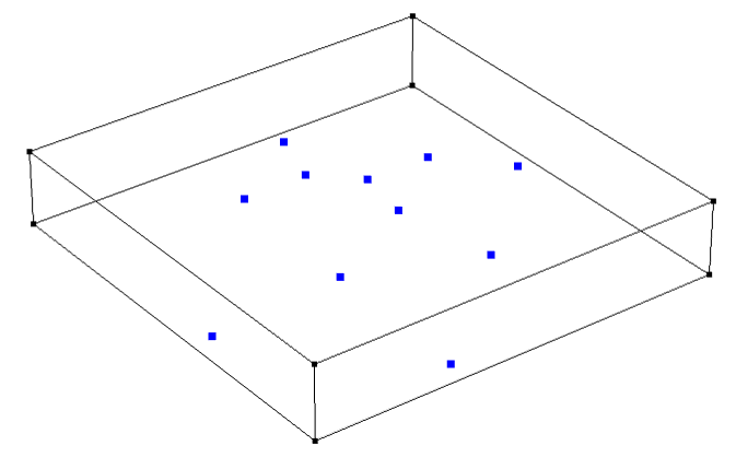
The data points and the bounding block.
Once the geometry is defined, we define an Integration Component Coupling operator over the points that we just created. Since the integration is done over a set of points, this operator is equivalent to taking a sum of an expression evaluated over the set of points. Next, we define three variables, as shown in the screenshot below.
First, the variable r = eps+sqrt((dest(x)-x)^2+(dest(y)-y)^2) will be used to compute the distances between all of the centers. Note the usage of the dest() operator, which forces the expression within the operator to be evaluated on the destination points instead of the source points. A very small nonzero term ( eps is machine epsilon) is added so that this expression is never precisely zero.
Next, the variable phi = r^2*log(r) is Equation (2), the thin-plate spline basis function. Note that this function converges to zero for a radius of zero, but we did need to make the radius very slightly nonzero because of the log function so that the basis function can be evaluated at zero. It is also worth remarking that this function could be changed to any other desired basis function.
Lastly, the definition RBF = intop1(w*phi)+a0+a1*x+a2*y is Equation (3), the interpolated surface itself, with weights that are not yet computed. Keep in mind that the integration component coupling operator takes a sum of the expression within the operator over those points.
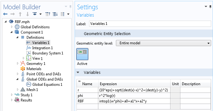
A screenshot showing the definitions of the variables.
Now that the geometry is set up and all variables are defined, we are ready to solve for the weights for the RBF and the polynomial terms. This is done with a Point ODEs and DAEs interface, defined over the points that we want to interpolate, as shown in the screenshot below. We can set all of the units to dimensionless, since the point locations are also dimensionless. These settings define a set of unknowns, w, which will have a different value for each point.
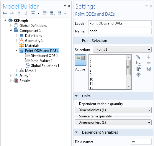
Settings for the Point ODEs and DAEs interface.
Within this physics interface, only two features need to be modified. Firstly, the settings for the Distributed ODE need to be adjusted as shown below. The Source Term is defined as z-RBF. Since all other terms in the equation are zero when a Stationary study is solved, this term means that RBF=z at all of the selected points. With this one feature, we define rows 1 through N of Equation (4).
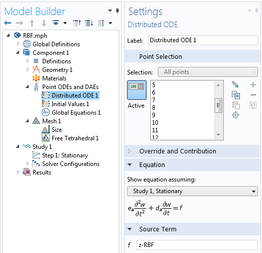
The settings for the Source Term at each point.
Secondly, we need to define the last three rows of Equation (4). This is done with a Global Equations feature, as shown in the next screenshot. These three equations solve for the weights a0, a1, and a2. Again, the integration coupling operator takes a sum of the expression over all selected points. With these two features, the problem is completely defined and almost ready to solve.
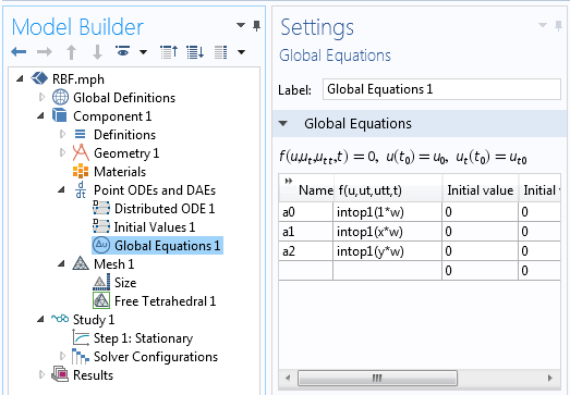
A screenshot showing the Global Equations for the polynomial weights.
Solving this model requires that we have a mesh on all points, so we apply a free tetrahedral mesh to the bounding box and then solve with a Stationary solver. Once the problem is solved, we can plot our interpolation function, the variable RBF, as shown below.
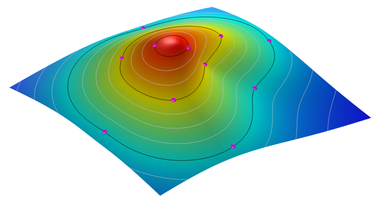
The smooth and differentiable interpolation surface passes through all of the data points.
Packaging the Functionality into a Simulation App
If you would like to use this functionality without setting up all of these features in your own models, you are also welcome to download our demonstration app from our Application Gallery, which takes in the xyz data points from a comma-delimited file and computes the interpolation surface. Up to 5000 data points can be interpolated with this demo app.
In addition to computing this surface, the app can write out the complete analytic function describing the surface, and also write out a COMSOL-format CAD file of the surface itself, all within the core capabilities of COMSOL Multiphysics. The CAD data is a NURBS surface and thus only approximately represents the function, but to a very high accuracy for reasonably smooth surfaces. A screenshot of the app’s user interface is shown below.
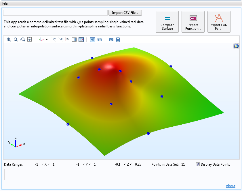
Screenshot of an app that computes an interpolation function and writes out the function and CAD surface.
Try It Yourself
Try calculating the interpolation between a set of points using a simulation app by downloading the demo app below:
Further Resources
If you’re interested in finding out more about the Application Builder and COMSOL Server™, which can be used to build and run this app, check out the resources below.
- Read a complete rundown of instructions in the Introduction to Application Builder manual
- Watch these videos to learn about how to use the Application Builder and COMSOL Server™
- Read these blog posts to see how simulation apps are used in a variety of applications
What would you like to do with COMSOL Multiphysics? Do you have further questions about the capabilities of Radial Basis Functions? Contact us for help.


Comments (4)
Dennis Nagy
March 17, 2016Wow! What goes around comes around. Bill Knudson and I developed software and published a paper on this approach in 1974! I’m sure the above approach must be better after 42 years.
http://www.freepaperdownload.us/1752/Article5135349.htm
Walter Frei
April 1, 2016 COMSOL EmployeeHi Dennis, Nice of you to post this interesting article. I think the advantage here is in the flexibility of using the output in other COMSOL models, either as a geometric surface, or as a function.
Peter Oving
December 6, 2018Hi Walter,
Thanks for your very interesting article!
I had liked to see the results of the application…
But the only file to download is a csv file.
To see how it works,.. is a little bit difficult with only the list of points.
Is there a possibility to get more information?
Sincerely yours
Walter Frei
December 6, 2018 COMSOL EmployeeHi Peter,
It is updated now to version 5.4.
Thanks,