Centre d'apprentissage

Tracking Eigenmodes in Parameter Sweeps

---

When performing an eigenfrequency analysis in conjunction with a parameter sweep, the mode solutions may not always be ordered by mode family. This becomes particularly evident when there are mode crossings or degeneracies in the linear system. Here, you will learn how to categorize eigenmodes using the mode overlap integral in COMSOL Multiphysics^®.

A Simple Example

Let's consider a relatively simple example: the 2D wave equation on an elliptical domain with fixed external boundaries (displacement ). We solve for the first five eigenmodes while sweeping the height of the ellipse. The width of the ellipse is fixed at , while the height  varies between 8 cm and 12 cm. In the middle of the parameter range , the simulation domain is a perfect circle, and the symmetry causes some eigenmodes to be mutually degenerate. The magnitude of displacement for each of the first five modes can be seen below.

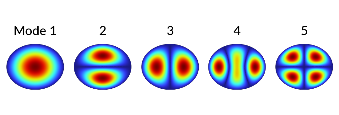
The first five eigenmodes while sweeping the height of an ellipse.

Note the mode crossing at when the natural frequencies are plotted against height.

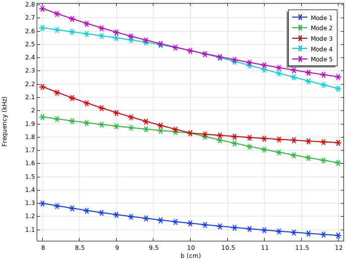
Eigenfrequencies of the 2D wave equation plotted against the height of the elliptical domain. Note the mode crossing at b = 10 cm.

Upon closer inspection, we find that modes 2 and 3 are mixed up post-crossing. This happens because the eigenvalues are colored according to their order in the solution dataset. To remedy this, we can use the mode overlap integral to categorize the mode solutions:

The equation above is defined in the most general sense, with and representing two arbitrary eigenmode solutions. The integrals are performed over the entire simulation domain, and the star suffix indicates complex conjugation. The numerator represents an inner product between the two modes, whereas the denominator normalizes the value of to lie between 0 and 1. For this specific problem, the overlap integral can be simplified to

In the following sections, we will demonstrate how to implement the overlap integral calculation to categorize modes. You can follow along by opening the starting model file here.

Defining a Mode Normalization Variable

The first step is to define a mode normalization variable so that it can be referenced later in the overlap integral calculation. The mode norm is mathematically defined as follows:

First, create an integration operator that covers the entire simulation domain.

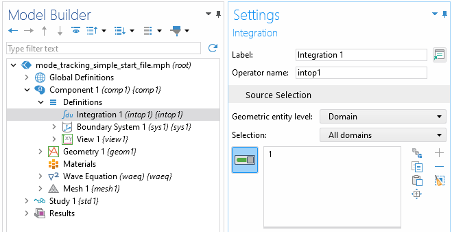
Settings window for Integration node.

Next, create a Variables node and define a modeNorm variable that uses the following expression:

intop1(u^2)

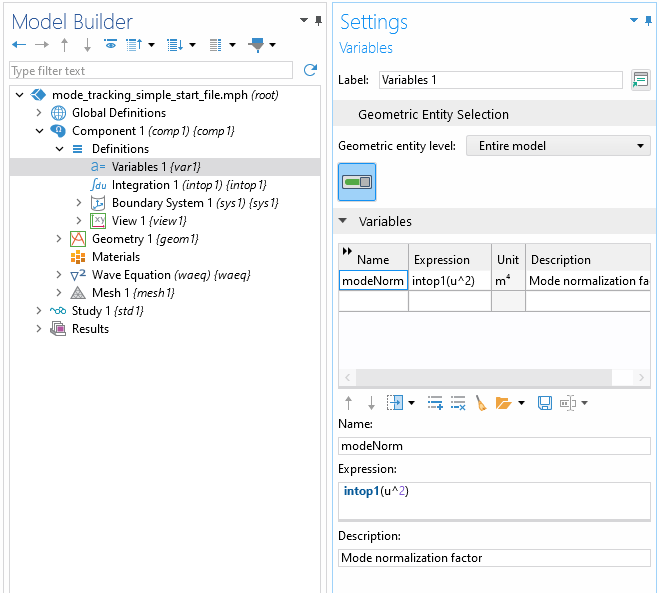
Settings window for Variables node.

Note that the appropriate expression will differ depending on the model physics and dependent variables. For instance, when the dependent variables are components of the electric field, then the integrand should define a dot product of the field with its conjugate.

After defining the modeNorm variable, compute the study.

Using the Join Dataset to Set Reference Modes

We will use the Join dataset to facilitate comparison between a particular mode solution (also known as the reference mode) and the complete mode solutions. The reference mode should be a solution that is representative of the tracked mode family.

After computing the study, right-click on Datasets and select Join. 

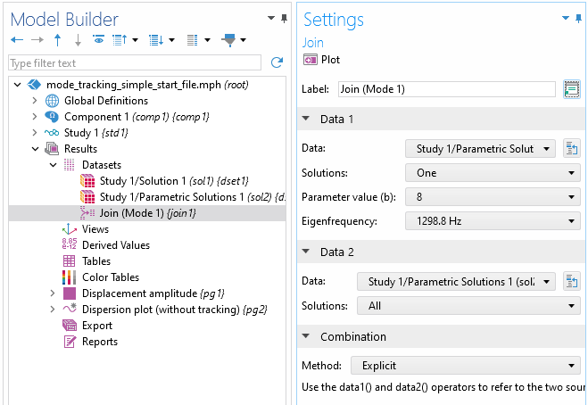
Settings window for Join node.

Set Data 1 to point to the reference mode. In this case, we select the first eigenmode for the case . Set Data 2 to point to the complete solution. For the combination method, choose Explicit. The explicit method allows us to reference specific variables in each solution using the data1() and data2() operators.

Calculating the Mode Overlap Using an Evaluation Group

Next, right-click on Results and add an Evaluation Group. Set the source dataset to the Join dataset. 

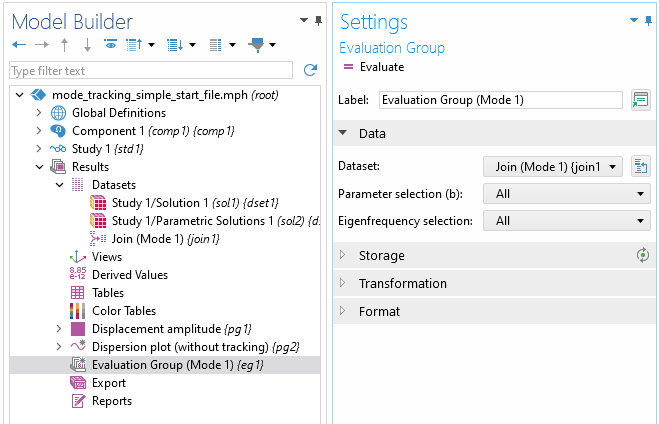
Settings window for Evaluation Group node.

Right-click on the new Evaluation Group node to add a Surface Integration subnode. (For 3D problems, replace Surface Integration with Volume Integration.) For selection, select All domains. The expression to be integrated is as follows:

 data1(u)data2(u)/sqrt(data1(modeNorm)data2(modeNorm))

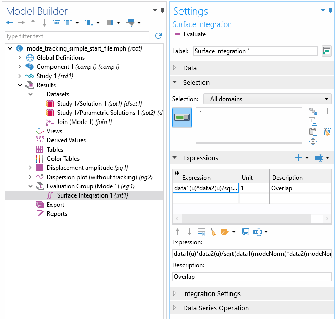
Settings window for Surface Integration subnode.

Here, data1(u) refers to the displacement of the reference mode, and data2(u) refers to the displacement of the other modes. In the denominator, we reference the mode normalization variable that we defined earlier.

Next, modify the Transformation settings in the Evaluation Group node settings, as shown in the following screenshot.

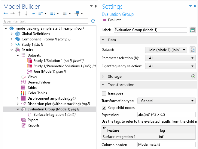
Settings window for Evaluation Group node Transformation settings. 

In the expression box, int1 refers the integral value calculated by the Surface Integration node, and abs(int1)^2 gives the value of as defined in equation 2. The intention here is to generate a new Boolean data column which indicates whether the overlap value is a match for the reference mode (1 is a match, 0 is not). Hence, there is a logical comparison between and a threshold value of 0.5 in the expression. 

Note that the threshold value is not fixed, but instead may vary from problem to problem or between different mode families. The goal is to pick a threshold value that cleanly separates solutions belonging to the desired mode family from the rest. In problems where there is a wide spread of mode overlap values, some fine-tuning via trial and error may be necessary.

In the Column header box, shown in the screenshot above, we can optionally give a title to this transformed data column. We can also check the Keep child nodes option to preserve the original overlap data column. When you are done, click the Evaluate button. Be aware that the calculation may take some time, especially for large models.

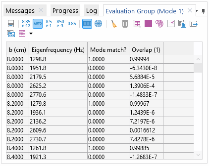
Table for Evaluation Group.

After evaluating, a table should display that looks similar to the above. If you wish to add more data columns the table, you may do so by adding additional evaluation nodes to the Evaluation Group. Remember to use the data1() and data2() operators to reference the appropriate mode solution.

Plotting with Table Graph

Create a 1D Plot Group and add a Table Graph node. 

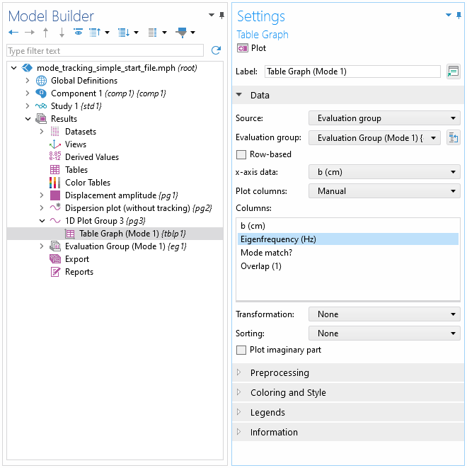
Settings window for Table Graph node.

For source, pick the newly created Evaluation Group. Select the appropriate x-axis data (swept parameter) and plot column (eigenvalue). Feel free to adjust the coloring, style, and legend options as desired. 

Next, right-click on the Table Graph node and add a Filter subnode. In the expression box, enter col3==1. Here, col3 refers to the mode match data column. 

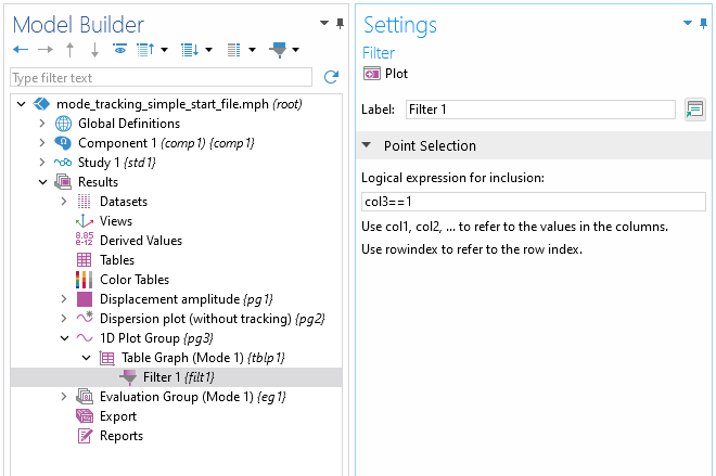
Settings window for Filter subnode.

The Filter subnode filters the plot data based on a given logical criteria. In this case, only the matched mode solutions are plotted. Click the Plot button to execute the plot.

Tracking Additional Mode Families

To track additional mode families, we simply repeat the previous steps. You can make use of the Duplicate action to quickly set up additional Join, Evaluation Group, and Table Graph nodes. To do so, right-click on the respective node and select Duplicate (CTRL-SHIFT-D shortcut). For each new mode family:

1. Duplicate the Join dataset. Rename the node and update the Data 1 section to point to a new reference mode.
2. Duplicate the Evaluation Group. Rename the node and change the source dataset to the new Join dataset. Click Evaluate to obtain the data table.
3. Duplicate the Table Graph node. Change the evaluation group source to the new evaluation group. Change color, style, and legend options as desired. Click Plot to update the plot.

You can also group nodes together to better organize the model tree. To do so, highlight all the nodes to be grouped, right-click and select Group (CTRL-G shortcut). 

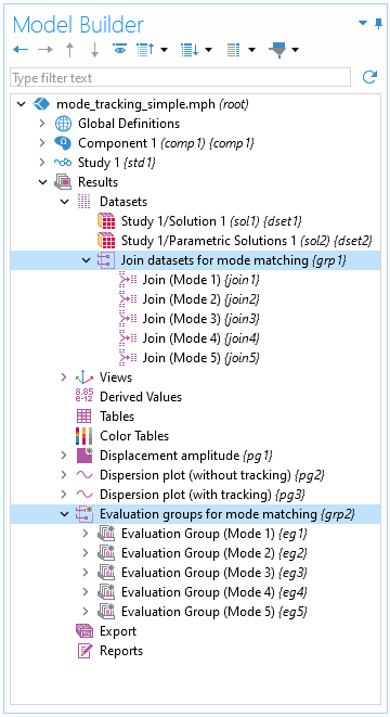
Model Builder tree showing groups for mode matching.

Important Usage Notes

• Remember to reevaluate each Evaluation Group after making any changes that would affect the mode match result. 
• After clearing solutions or making significant changes to the eigenfrequency study, it is sometimes necessary to set up the reference modes in the Join dataset(s) again. For better reproducibility, we recommend keeping track of the reference mode used for each Join dataset in an external document.
• Regarding the choice of reference mode, we recommend choosing a mode that overlaps well with the rest of the modes in its family, while having little resemblance to the remaining modes. Usually this can be determined visually by plotting the mode solutions. If a mode family evolves significantly over the parameter range, some trial and error may be needed to find the appropriate reference mode.

Further Learning

Check out this blog post for a demonstration of mode tracking applied to various physics applications. To learn more about the Join dataset and its various other uses, see this blog post.