Centre d'apprentissage

More on PCE Surrogate Models in Two Variables

---

Continuing the discussion on Polynomial Chaos Expansion (PCE) surrogate models from Part 7, we will now build upon the example from that article, which dealt with a single random variable, and we will introduce a second random variable with a different probability distribution. The introduction of a second random variable leads to interaction terms in the PCE representation. As in Part 7, we will calculate the PCE for an analytical function and compare with direct Monte Carlo simulations.

Polynomial Chaos Expansion in Two Variables

Let's now consider a case with two input parameters and one quantity of interest, or output parameter. Assume that we have a function

that we want to represent with a polynomial chaos expansion (PCE). In general, this function might be defined by the solution to a finite element model. Further, assume that the input parameters and have certain probability distributions. We introduce random variables and that represent the stochastic properties of and . We can represent the function as:

where and are orthogonal polynomials associated with the random variables and , respectively, with given probability distributions, and are the coefficients to be determined.

Just as in the univariate case, the coefficients are determined by projecting the function onto the orthogonal polynomial basis:

where the inner products are defined as:

where is the joint probability density function of and .

When the random variables and are independent, their joint probability density function can be factorized into the product of their marginal densities:

This assumption is frequently made when working with PCE models, and we will use this assumption here.

If we work with a normalized basis, we get:

where

and

and

Just as in the univariate case, when using the built-in PCE surrogate model functionality, the inner product integrals are not computed. Instead, the coefficients are found using a least-angle regression method. However, for simple analytical functions, these integrals can be computed by hand, as illustrated by the example in the next section.

An Analytical Example in Two Variables

Let's see how to approximate with PCE where is a random variable that is uniformly distributed over the interval and is a random variable with standard normal distribution.

The polynomials that are orthogonal with respect to a uniform probability distribution on are the Legendre polynomials, denoted , as covered in More on PCE Surrogate Models. The polynomials that are orthogonal with respect to a standard normal probability distribution are the Hermite polynomials, denoted .

The first few unnormalized and normalized Hermite polynomials are listed in the following table:

n
0
1
2
3
4

The PCE approximation

now becomes:

or, expanded out and showing a few of the terms:

Computing these coefficients by hand is very tedious. In general, we have to compute the integrals:

where

and

Let's just compute one of the coefficients:

It turns out that many of the other lower-order coefficients are zero. In fact, for degrees lower than or equal to , the only other nonzero coefficient is: .

So, a low-order PCE approximation to the random function is:

The fact that many of the low-order terms are zero or near-zero is common in practice for PCE surrogate models. Due to this, the representation used in COMSOL Multiphysics^® is a sparse polynomial chaos expansion (SPCE) where only the most significant terms are kept. This is covered in more detail in More on Sparse PCE Methods.

Mean and Variance Calculation

Just as in the one-variable case, we can compute the mean and variance.

The mean is equal to the lowest order coefficient, which is zero:

The variance is the sum of squares of the other coefficients:

For the approximation used here we get:

The standard deviation is:

Uncertainty Quantification Module Calculations

For comparison, we can perform an uncertainty propagation analysis for the function . The resulting QoI Confidence Interval table below shows a mean value near zero and a standard deviation of about 0.703, which is consistent with the analytical calculations.

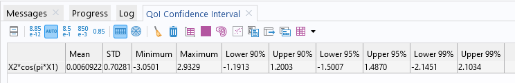The QoI Confidence Interval table results.

The PCE surrogate model created using the built-in adaptive method agrees well with the original function , as shown in the visualization below.

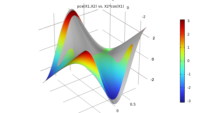A warped surface plot displaying a rainbow color distribution and warped appearance. A comparison between the PCE surrogate model function ( Rainbow color table) and the function (gray).

In addition, we can perform direct Monte Carlo simulations using the same technique as covered in the tutorial model based on the Ishigami function.

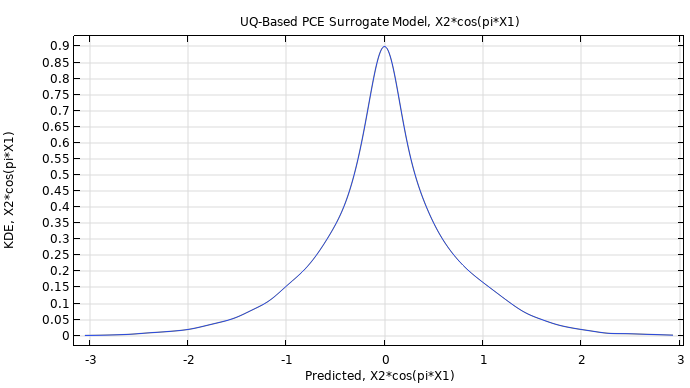
The table below compares the estimated probability distributions (KDE plots) of from two direct Monte Carlo simulations and a UQ-based PCE surrogate model with an uncertainty propagation analysis. T he lower frequency content of the distribution is well-represented by the expansion with reasonably accurate values for quantities such as the mean and variance. The built-in automatic PCE regression method can find a good fit using only 100 sample points, whereas the Monte Carlo simulations here use 30,000 sample points. The fact that PCE surrogate models can be created using orders of magnitude fewer sample points is the main motivating factor for using it instead of direct Monte Carlo simulations. In a case where the model evaluations are not an analytical function, such as , but instead a full-fledged finite element model, it is important to keep the number of model evaluations to a minimum. The default settings for the PCE surrogate model minimize the number of model evaluations. For more details, see More on Sparse PCE Methods.

Plot	Comments
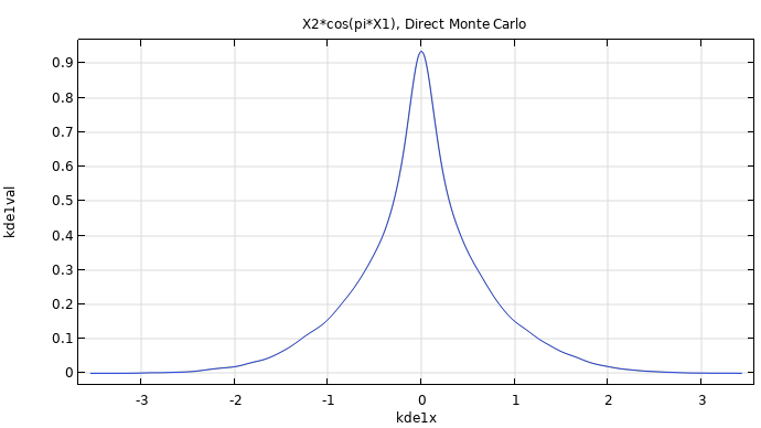
	The figure shows a KDE plot of a PCE surrogate model computed using the Adaptive sparse polynomial chaos expansion method in the Uncertainty Quantification Module. This PCE includes higher-degree terms, compared to the analytically derived PCE surrogate model, which only includes terms up to degree (4,4). The corresponding model file is available here.
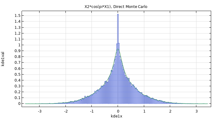
	The figure shows a KDE plot of a Monte Carlo simulation of the analytically derived PCE, , including terms up to degree (4,4). The plot is based on 30,000 sample points for . The corresponding model file is available here.
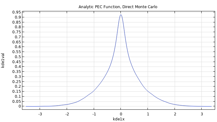
	The figure shows a KDE plot of a Monte Carlo simulation of the function , without PCE approximation. The plot is based on 30,000 sample points for . The corresponding model file is available here.
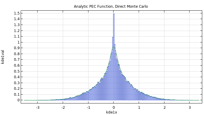
	The figure shows a histogram plot of a Monte Carlo simulation of the analytically derived PCE,, including terms up to degree (4,4). The plot is based on 30,000 sample points for . The corresponding model file is available here.
	The figure shows a histogram plot of a Monte Carlo simulation of the function , without PCE approximation. The plot is based on 30,000 sample points for . The corresponding file is available here.