Calculating the Large-Signal Parameters of a Speaker Driver from FEA
The small-signal parameters derived in Part 6 are sufficient for describing the driver's behavior in the low-frequency limit when the coil displacement from its equilibrium position is small and the problem stays linear. However, when the displacement of the voice coil becomes large for higher voltage excitation, the linear assumption is not valid anymore and the lumped parameters' dependency on coil displacement needs to be taken into account. In this part of the course, we discuss how to estimate the large-signal parameters of a speaker driver when large displacements are applied to the voice coil.
Nonlinear Mechanical Compliance Calculation
To obtain the nonlinear mechanical compliance,  , as a function of coil displacement,
  , for large deformations, we can adopt the same physics setup and study steps as used in the linear mechanical compliance analysis for small deformations (see Part 6) with the following two changes:
- Enable a geometrically nonlinear analysis for the structural analysis by selecting the Include geometric nonlinearity checkbox in the Study Settings section of the Stationary study step, as seen in the image below. This enforces the study to use a large strain formulation, which is required when the structure experiences large deformations.
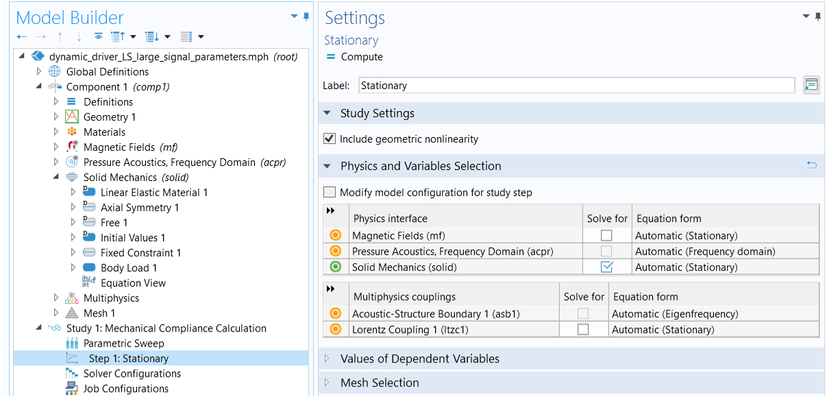 A Stationary study showing the Include geometric nonlinearity checkbox selected and Solid Mechanics as the selected physics.
A geometrically nonlinear analysis is necessary for large deformations.
A Stationary study showing the Include geometric nonlinearity checkbox selected and Solid Mechanics as the selected physics.
A geometrically nonlinear analysis is necessary for large deformations.
- Use range functions to change the value of the applied body load in the Study Settings section of the Parametric Sweep settings, as seen below. For small deformations/linear analysis, two points are sufficient for calculating the compliance. However, for large deformations, the compliance will change at different displacement, and thus the study needs to cover the full range of forces that would displace the coil from zero up to the largest offset. Two range functions are used here: range(0,2,20) covers the cases when the coil moves upward, and range(0,-2,-20) when the coil moves downward.
 The displacement range is defined in a Parametric Sweep window associated with a Mechanical Compliance study.
The structural analysis is run through the full displacement range in order to get the nonlinear mechanical compliance curve.
The displacement range is defined in a Parametric Sweep window associated with a Mechanical Compliance study.
The structural analysis is run through the full displacement range in order to get the nonlinear mechanical compliance curve.
After solving the study, we can conduct a point evaluation on a point in the coil domain to get the coil displacement versus the applied force, as shown below.
 A Point Evaluation Settings window showing expressions for displacement and force and a table of values.
The displacement vs. force data is evaluated at a point in the coil domain and saved to a table.
A Point Evaluation Settings window showing expressions for displacement and force and a table of values.
The displacement vs. force data is evaluated at a point in the coil domain and saved to a table.
The compliance can be calculated by evaluating d(w)/d(Fcom), the derivative of the displacement with respect to the applied force. Since differentiation can't simply be done over the discrete points in a table, we can turn the table into a smoothed function in order to apply the differentiation operation inside COMSOL Multiphysics®. In order to do this, we need the following steps:
- Generate an interpolation function using the displacement-force data saved in the Result table from Evaluation Group 1, as shown in the image below. Here, the function is named Force, and the Cubic spline option is selected for the Interpolation feature, and Linear is selected for Extrapolation. It is also important to make sure that the units are defined correctly for both the function and the argument.
 An interpolation feature uses displacement-force data from a table of values and plots the interpolation.
The displacement-force data saved in the table is used directly to define an interpolation function.
An interpolation feature uses displacement-force data from a table of values and plots the interpolation.
The displacement-force data saved in the table is used directly to define an interpolation function.
- Define a Grid 1D dataset. Use the Study 1 solution as the source data and set the parameter x to range from -5.77 mm (about the largest downward displacement) to 6.11 mm (about the largest upward displacement) so that it covers the coil displacement band found in the study. This parameter x can then be used as the argument for the Force function.
 A Grid 1D dataset is configured with the displacement parameter of interest and associated bounds.
The Grid 1D dataset defines a parameter that covers the displacement range found in the study.
A Grid 1D dataset is configured with the displacement parameter of interest and associated bounds.
The Grid 1D dataset defines a parameter that covers the displacement range found in the study.
- Go to the Study 1 node and click Update Solution. This makes the Force function available in results evaluation.
Then you are ready to calculate the displacement-dependent stiffness,  , and compliance, , as shown in the image below. Using the Grid 1D dataset as the source data, a line plot of d(Force(x),x) gives the stiffness (top), and its inverse gives the compliance (bottom). A factor of 1000 is used for the compliance plot so that it is shown in the unit of mm/N.
 Two Line Graph features are used to plot the stiffness and compliance vs. the displacement of the coil.
The stiffness (top) and compliance (bottom) as a function of coil displacement.
Nonlinear Electrical Parameter Calculation
To obtain the electrical parameters as a function of coil displacement, we can use a quasi stationary analysis of the electromagnetic components of the speaker driver. That is, we will move the coil, run the study, and calculate the electrical parameters at each coil displacement. The geometry needs some modification so that the coil can be displaced for each run.
The new geometry for this analysis can be constructed in a new component, Component 2, as shown in the image below. The new geometry contains only the coil, magnet, soft irons, and the air domain. A Move operation is used to move the coil in the z direction, and the displacement from its original position is controlled by a parameter named zoff.
 A Move geometry feature has the cross section of the coil as an input shown in blue.
The coil domain can be moved in the new geometry for a quasi stationary analysis.
A Move geometry feature has the cross section of the coil as an input shown in blue.
The coil domain can be moved in the new geometry for a quasi stationary analysis.
We only need the Magnetic Fields interface in this analysis, and the setup of the physics is the same as that in Component 1. To extract  as a function of coil displacement, run a Stationary study of the magnetic field and use a Parametric Sweep to change the position of the coil, as shown in the image below. This is solved in Study 2 of the attached model.
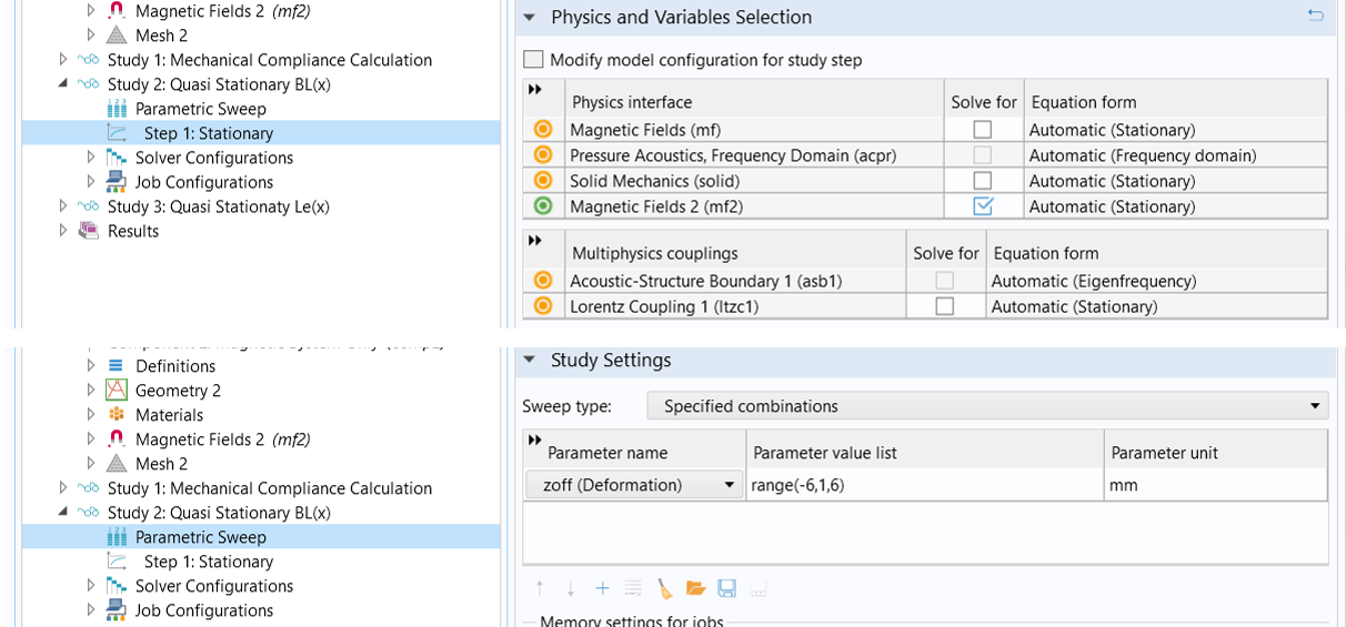 The study settings are shown via the Stationary step and Parametric Sweep Settings windows.
Study settings for extracting force factor (BL) as a function of coil displacement.
The study settings are shown via the Stationary step and Parametric Sweep Settings windows.
Study settings for extracting force factor (BL) as a function of coil displacement.
Similar to the method we used in Part 6, we can calculate  by evaluating the surface average of the term
  over the coil domain for each displacement. Instead of using a Global Evaluation node under Derived Values and saving the results to a table, we define an average operator over the coil domain under Component 2 > Definitions, as seen below.
 The configuration for an Average feature used as part of the force factor calculation is shown.
An average operator is defined over the coil domain for calculating BL.
The configuration for an Average feature used as part of the force factor calculation is shown.
An average operator is defined over the coil domain for calculating BL.
Evaluation of aveop2(-mf2.Br*N0*2*pi*r) gives the  value, the result of which is shown below.
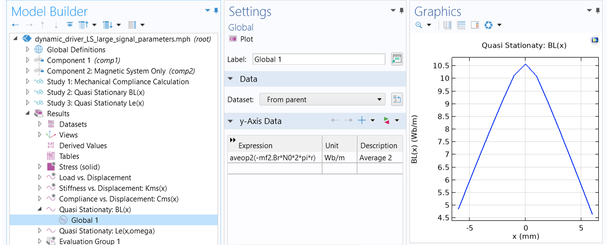 A global feature using the values from Average 2 as part of the BL calculation and plotting the result.
Force factor (BL) as a function of coil displacement.
A global feature using the values from Average 2 as part of the BL calculation and plotting the result.
Force factor (BL) as a function of coil displacement.
The extraction of coil inductance requires a Small-Signal Analysis, Frequency Domain study. Again, it includes two steps: a Stationary step where the stationary magnetic field generated by the permanent magnet is calculated, and a Frequency Domain Perturbation step, where the voice coil is excited with a harmonic AC voltage, and where the perturbated magnetic field and the additional currents induced in the electromagnetic circuit are solved. These steps are solved in Study 3, as shown below. Here, a Parametric Sweep is also used to change the position of the coil.
 The study settings in the Stationary, Frequency Domain Perturbation, and Parametric Sweep Settings windows for extracting coil inductance vs. coil displacement.
Study settings for extracting coil inductance (Le) as a function of coil displacement.
The study settings in the Stationary, Frequency Domain Perturbation, and Parametric Sweep Settings windows for extracting coil inductance vs. coil displacement.
Study settings for extracting coil inductance (Le) as a function of coil displacement.
The coil inductance is calculated internally and saved in the variable named mf2.LCoil_1. It is a function of both coil displacement and frequency. A plot of its magnitude is shown below.

Coil inductance (Le) as a function of coil displacement and driving frequency.
Envoyer des commentaires sur cette page ou contacter le support ici.