Centre d'apprentissage

Creating a Multiphysics-Driven Gaussian Process Surrogate Model

---

To create a Gaussian Process (GP) surrogate model, we will continue working with the thermal actuator tutorial model and dataset from Part 3 of this course. In this part, we will focus on the practicalities of adding and training a Gaussian Process function. For more information, the theoretical background and settings for this type of surrogate model are covered in a separate resource discussing Gaussian Process surrogate models.

Note: This example and demonstration requires the Uncertainty Quantification Module.

Gaussian Process Model Overview and Comparison to Deep Neural Network Model

GP surrogate models are based on a generalization of linear regression called Gaussian process regression, or GP regression for short. Another name for this method is Kriging, a method rooted in geostatistics, particularly in gold ore prospecting in the 1950s. The goal was to develop a statistical method that could make reliable predictions based on very few measurements, or samples. Generally, a GP surrogate model should be considered instead of a deep neural network (DNN) model if:

• Model computation is expensive, and you can only afford to compute a small number of data points (input parameter–output value sets)
• You want to avoid defining a surrogate model such as a DNN with layer architecture by trial and error
• You have fewer than a few thousand data points
• You want to estimate uncertainty in the model

The GP surrogate model has a default limit of 2000 data points due to the underlying algorithm's constraints. However, you can increase this limit slightly, depending on the computational power of your computer. In contrast, the DNN surrogate model has no such limitation and can be trained on millions of data points. However, while a DNN model requires testing many network architectures, a GP model works with less user input and provides well-calibrated uncertainty estimates.

Building a Gaussian Process Surrogate Model

Continue working with the model from Part 3. If you have access to the Uncertainty Quantification Module, then you can add a GP surrogate model function through the Global Definitions node by clicking Functions and selecting Gaussian Process.

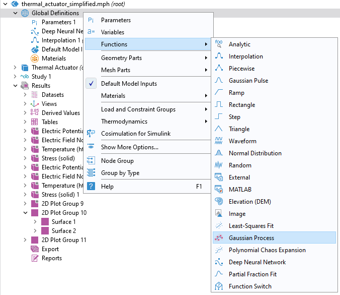
Adding a Gaussian Process function.

In the Data section settings for the Gaussian Process function, select Results table as the Data source and make sure the Result table is set to Design Data. This will enable you to use the same dataset that we used for the Deep Neural Network function in Part 3. The Data Column Settings will automatically be filled out with the correct names for Argument and Function values: L, DV, and comp1.point1 for the actuator length, applied voltage, and Point Probe, respectively. The default name for the Gaussian Process function is set to gpm1.

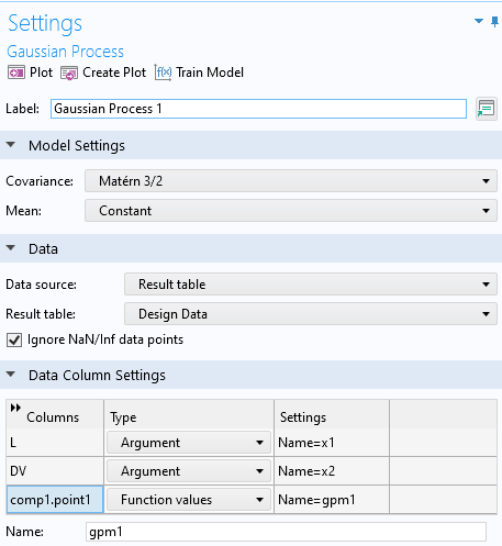
The settings for the Gaussian Process function.

The Ignore NaN/Inf data points checkbox is selected by default and ensures that the training doesn't stop if the data table contains entries with Not a Number (NaN) or infinite (Inf) values. This can be the case, for example, when the physical model used to generate the data didn't converge for certain input parameters.

We have now defined all the settings we need before training. Click Train Model at the top of the Gaussian Process function Settings window. The training is almost instantaneous since we only have 50 data points.

For function visualization, we will make a copy of a previous Surface plot and modify the settings. To do so, right-click 2D Plot Group 11 > Surface 2 and select Duplicate. Change the Expression to gpm1(x1,x2) and click Plot. Change the Color table to Magma, for example, to more easily identify the different plots. The functions are near identical except for in one corner where the automatic DOE sampling didn't quite reach the corner when using only 50 data points. You can also easily visualize just the Gaussian Process function by disabling the first two Surface plots.

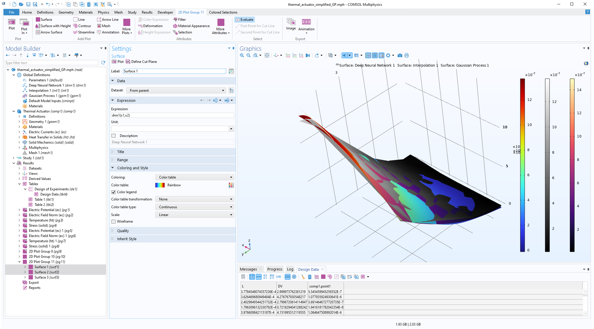The Model Builder with the Surface 1 plot selected under the 2D Plot Group 11 node and the corresponding Settings window and Graphics window displayed. The Graphics window shows a rectangular-shaped surface plot in 3D space that partially displays a rainbow color distribution from dark red to dark blue, partially displays a grayscale color distribution from white to black, and partially displays a heat camera color distribution from dark purple to a light yellow.

Visualizing the Gaussian Process function alongside the linear interpolation and DNN functions.

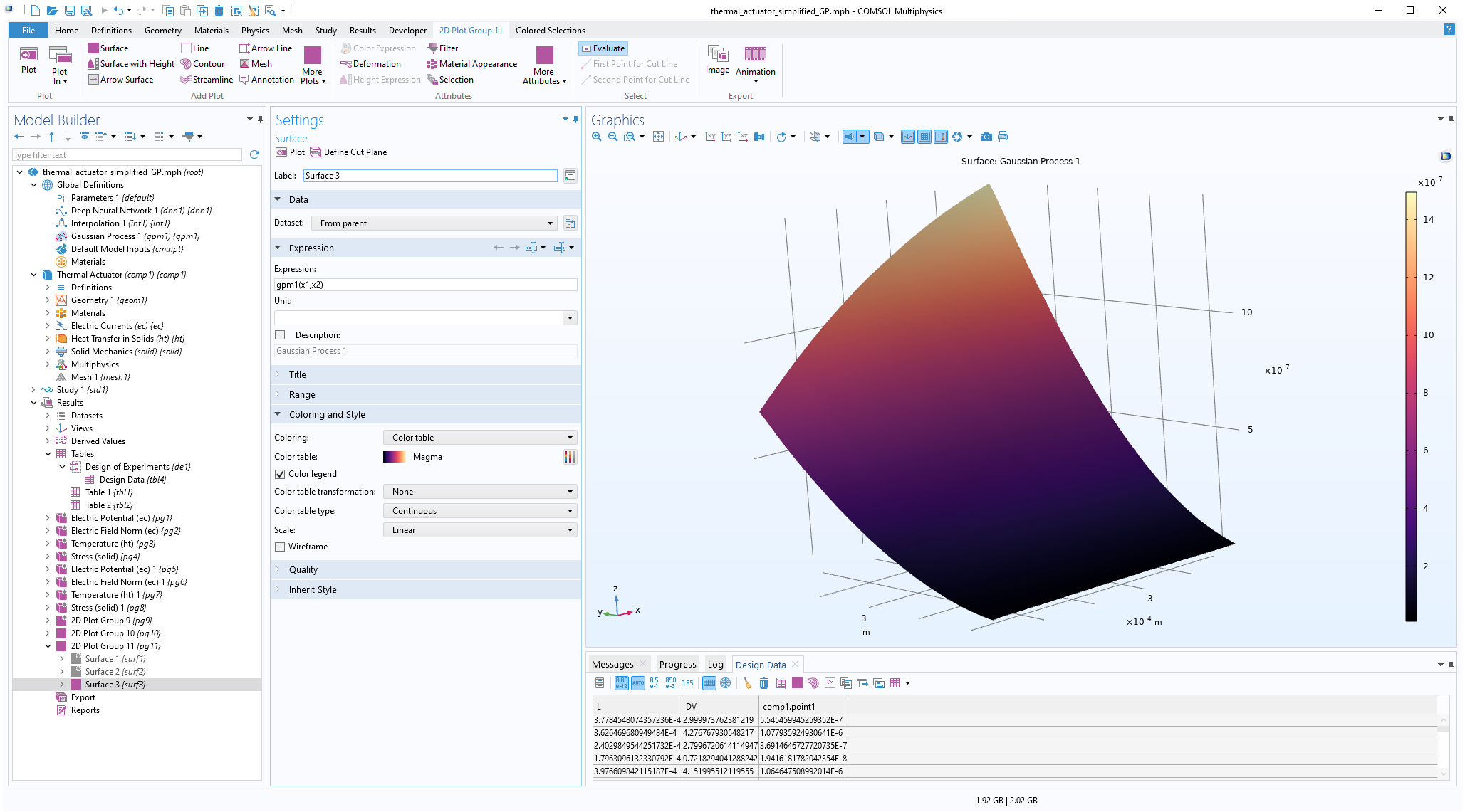The Model Builder with the Surface 3 plot selected under the 2D Plot Group 11 node and the corresponding Settings window and Graphics window displayed. The Graphics window shows a rectangular-shaped surface plot in 3D space that displays a heat camera color distribution from dark purple to a light yellow.

Visualizing the Gaussian Process function.

Model Uncertainty

In order to assess the uncertainty in the model, we can visualize the estimated standard deviation. To do this, go back to the Gaussian Process function window. In the Related Functions section, select Define standard deviation function. This makes a gpm1_stddev function available that can be visualized and evaluated just like any other function.

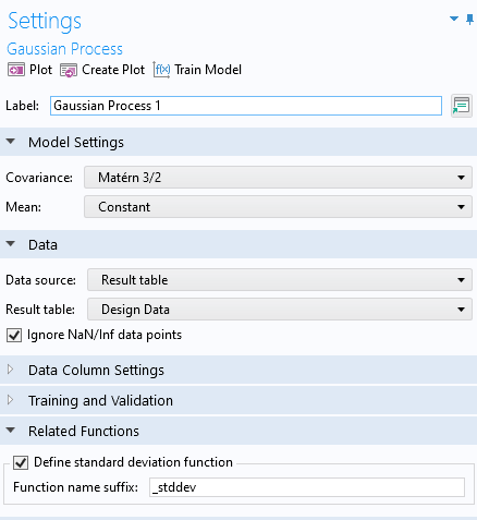
Enabling the standard deviation function for the Gaussian Process function.

To visualize the standard deviation estimator, in Results click Surface 3 > Hight Expression for the Gaussian Process visualization plot group. Change the height data setting to Expression and type gpm1(x1,x2). Now, click the Surface 3 plot and change the expression to gpm1_stddev(x1,x2). These settings will display the function value as a height and the standard deviation as a color. At this stage, you can also disable the Surface 1 and Surface 2 plots. In this case, change the Color table to Thermal for a clearer visualization. The uncertainty will be the lowest at the DOE sampling points, which in this visualization can be seen in darker color.

The Model Builder with the Surface 3 plot selected under the 2D Plot Group 10 node and the corresponding Settings window and Graphics window displayed. The Graphics window shows a surface plot with a rectangular shape that displays orange for the majority of the surface area and contains many dark red dots throughout.

The standard deviation function for the GP function.

To instead visualize the standard deviation in nanometers, change the expression to 1e9*gpm1_stddev(x1,x2). The maximum standard deviation value is about 9 nanometers, as shown in the figure below. To enable the display of maximum and minimum values in the color legend, select the Show maximum and minimum values checkbox in the 2D Plot Group 11 node.

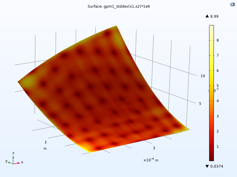
The standard deviation plot scaled to nanometers. A thermal color table is used.

The standard deviation values give an estimate of the uncertainty of the fit z=f(x1,x2) at each point (x1,x2) and is one of the advantages of a GP-based surrogate model. This type of uncertainty estimate is not available for the DNN surrogate model.

A GP surrogate model has a statistical interpretation where the function gpm1(x1,x2) is the predicted mean value of the model; there is one mean value at each input parameter pair. The standard deviation values represent the model's uncertainty about this predicted mean function. A higher standard deviation indicates greater uncertainty, while a lower standard deviation indicates higher confidence in the prediction. In regions where there are more data points (also called training data points) there will generally be a lower standard deviation because the model is more confident in its predictions in these areas. Conversely, in regions with fewer or no training data points, there will typically be a higher standard deviation, indicating that the model is less certain about its predictions in these areas.

The standard deviation can be used for confidence intervals around the predicted mean. For example, a 95% confidence interval for the prediction at a point (x1,x2) is given by [gpm1(x1,x2)-1.96*gpm1_stddev(x1,x2), gpm1(x1,x2)+1.96*gpm1_stddev(x1,x2)].

This interval represents the range within which the true function value is expected to lie with 95% confidence. The value 1.96 approximately corresponds to the point for which the cumulative distribution function, of a normal distribution, equals 0.975.

In addition to the density of data points, the uncertainty estimates depend on the choice of covariance function. For more information on covariance functions and the statistical properties of a GP surrogate model, see this resource on covariance functions.

Adaptive Gaussian Process

The standard deviation indicates an error boundary around the predicted values. A high standard deviation suggests that the true value could significantly differ from the predicted mean function, highlighting the need for more data points. The Uncertainty Quantification Module includes a solver option that capitalizes on this to select new sample points. The Adaptive Gaussian process method available in the Uncertainty Quantification study adaptively inserts new sample points in the input space where the confidence is low. Let's see how to use this option for the thermal actuator example, building on the previous example.

Right-click Study 1 and select Uncertainty Quantification > Uncertainty Quantification.

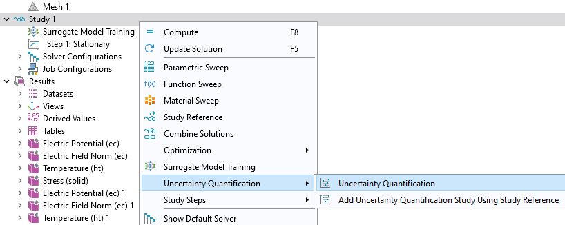The model tree with the Study 1 node selected and the corresponding menu shown, with the Uncertainty Quantification section expanded and the Uncertainty Quantification study selected.

Adding an Uncertainty Quantification study.

This study requires removing the Surrogate Model Training study. Click Yes in the dialog that asks you if you want to remove the Surrogate Model Training study.

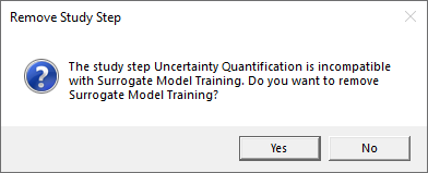
Replacing the Surrogate Model Training study with the Uncertainty Quantification study.

The Uncertainty Quantification study has similarities with the Surrogate Model Training Study in that it requires you to define Quantities of Interest and Input Parameters. Furthermore, it uses the same type of design of experiments method for sampling in the input space. The Uncertainty Quantification study includes five different study types, and we will select Uncertainty propagation from the UQ study type menu. To learn more about these study types, see the Learning Center entry "Using Uncertainty Quantification to Model Frequency Variation in a MEMS Resonator".

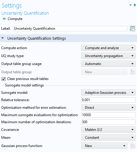
The Uncertainty Quantification study settings with the Uncertainty propagation and Adaptive Gaussian process options selected.

Make sure that you have selected the Uncertainty propagation option. The default Surrogate model type for Uncertainty propagation is Adaptive Gaussian process. Just like in the Surrogate Model Training case, enter comp1.point1 as the Expression for Quantities of Interest and L and DV for the Input Parameters. In this case, we stick to SI units. The Lower bound and Upper bound are: [150e-6, 400e-6] for the length, L, and [0.5,5] for the applied voltage, DV.

The Distribution setting is set to Uniform, which is the only option that makes sense in the example where we would like to create a surrogate model that can be used equally well in any part of the parameter space. However, when performing an uncertainty quantification analysis, it can be relevant to change this to, for example, a Normal distribution, in case your input variable follows this statistical distribution. The Uncertainty Quantification study settings are shown in the figure below.

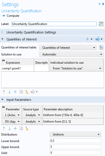
The Uncertainty Quantification study settings for the Adaptive Gaussian process.

Click Compute to start the adaptive process, which will take a few minutes of computation time. By default, the maximum number of sampled points (computed solutions) is set to 40. You can change this setting in the Input parameters sampling settings section.

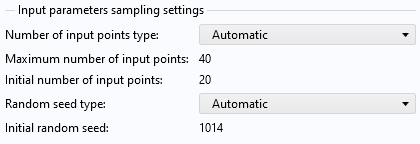
The input parameters sampling settings.

The Uncertainty Quantification study will automatically create and train a new GP model and place it under Global Definitions > Functions.

In the case of an Uncertainty Quantification study, the sampled variables are output to a Quantities of Interest table, rather than a Design Data table.

When the computation is finished, the plot shown is a kernel density estimation (KDE) plot of the probability density function estimate for the maximum displacement, as shown in the figure below. This plot shows which maximum displacement values are most likely to occur when the input parameter space is uniformly sampled within the set parameter boundaries.

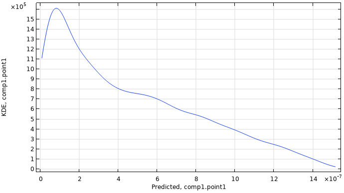
A KDE plot showing the probability density function estimate for the maximum displacement.

The figure below shows a comparison of the 50 data point nonadaptive GP function versus the 40 data point adaptive GP function. They are nearly indistinguishable. In a scenario with many input parameters (a large input parameter space), the adaptive method will typically be much more efficient. Note that in this case, all of the computations were done with SI units to keep things simple.

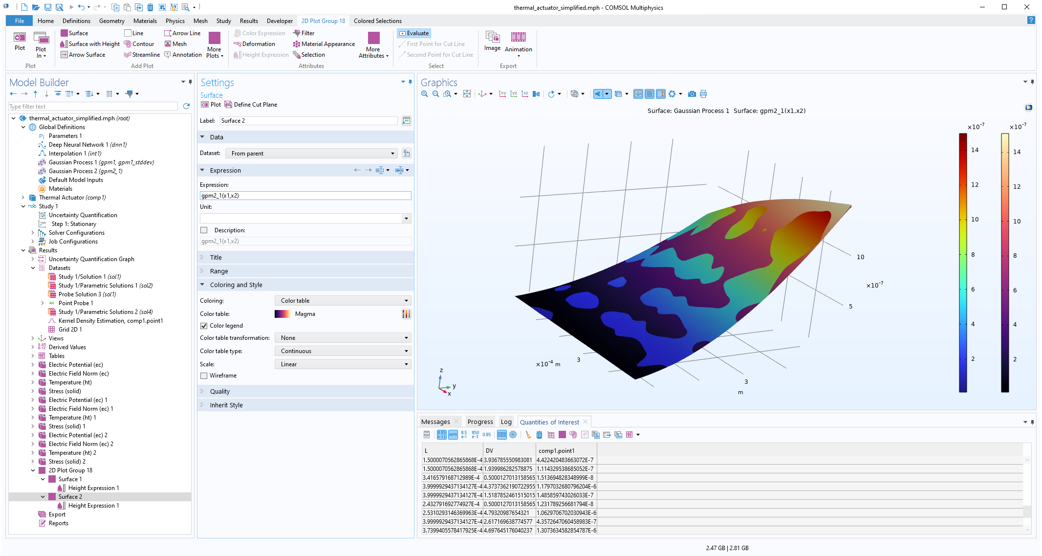The Model Builder with the Surface 2 plot selected under the 2D Plot Group 18 node and the corresponding Settings window and Graphics window displayed. The Graphics window shows a rectangular-shaped surface plot in 3D space that displays a rainbow color distribution varying from dark blue to dark red and a heat camera color distribution varying from dark purple to a light yellow.

A comparison of the nonadaptive and adaptive GP functions.

Just as in the previous case, we can plot the standard deviation. To do so, select the Define standard deviation function checkbox in the Related Functions section of the Gaussian Process function Settings window. Then, train the model and create a plot with the GP function as the height expression and the standard deviation function as the Surface plot expression. Change the color table to Thermal, as shown in the figure below. In this visualization, like in the previous example, the Surface plot expression has been multiplied by 1e9 to scale to nanometers. This allows us to see where the adaptive sampling points were chosen as the locations with darker color. We can also see that the adaptive approach gives us a model with higher confidence than previously, with a maximum standard deviation of about 5.6 nm versus the earlier 10 nm.

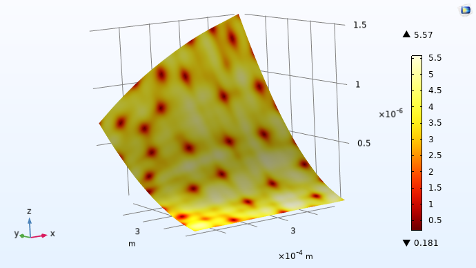
The standard deviation function for the adaptive Gaussian process.