Centre d'apprentissage

Performing a Screening Analysis UQ Study

---

This part of the course, along with several subsequent parts, will demonstrate how to use the Uncertainty Quantification Module to conduct a series of studies for a steel bracket model. We will begin by introducing the steel bracket model and performing a screening analysis to identify the input parameters that most significantly influence the quantity of interest. For a theoretical background on the numerical methods used for screening, see Supplement A in this course.

Steel Bracket Model Overview

The model used in this example is a specific type of steel bracket. This bracket is designed to install an actuator, which is secured on a pin positioned between the two holes in the bracket arms. The design objective is to ensure that the actuator's horizontal misalignment angle is not too large.

Bracket geometry with the quantity of interest, the misalignment angle, indicated.

The geometry of this example is created using the 3D fillet functionality that is available in the Design Module. A version of the geometry that does not include the 3D fillets can also be found here if you do not have access to the Design Module. The modeling instructions for this version are almost identical to the instructions for the version with fillets, though a few of the model parameters are slightly different, and the results differ somewhat between the two versions.

The geometry discussed in this article is fully parametric, with the parameters defined in the table below, accessible under Global Definitions > Parameters. We are interested in analyzing the bracket's performance when considering manufacturing variabilities in these nominal geometry parameter values.

Geometry parameters for the steel bracket model.

The mesh is customized so that the thickness of the material spans two tetrahedral elements, as shown in the figure below. Note that during the uncertainty quantification (UQ) calculations, the mesh will automatically regenerate for each new value of the geometry parameters.

The mesh for the steel bracket.

In this static analysis, the mounting bolts are assumed to be fixed and securely bonded to the bracket. One arm is subjected to an upward load, while the other experiences a downward load. These loads are applied as pressure on the inner surfaces of the holes, with an intensity of , where is the angle relative to the direction of the load resultants, as shown in the figure below.

The loads applied to the steel bracket. Upon computing the model, this plot is available by adding a predefined plot under the Results node and adding the Boundary Loads plot.

This force is assumed to remain constant in the uncertainty quantification studies. Likewise, the material properties of the generic structural steel are also considered invariant. The misalignment angle is selected as the quantity of interest (QoI). The design objective is to ensure that the actuator's horizontal misalignment angle, , does not exceed 0.1 degrees. The angle is defined as a variable, as shown in the figure below. Note that the unit conversion [1/deg] ensures that the angle phi is defined in degrees (and not radians).

The misalignment angle defined as a variable in terms of the z-location of the pin hole centers.

The corresponding model file with the static analysis is available for download here. This file will be used as the starting point for the UQ analysis, starting with screening in the next section.

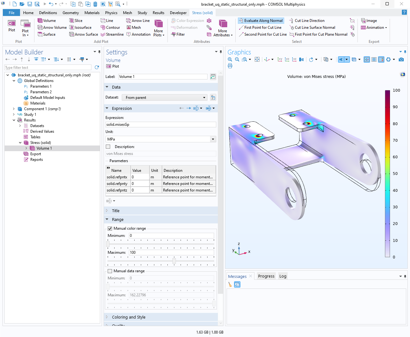The Model Builder with the Results node for visualizing the stress selected, the corresponding Settings window, and the corresponding plot displayed in the Graphics window.

The stress results from the static structural analysis of the steel bracket.

Screening Analysis

The first step of a UQ analysis is to determine which of the input parameters have the greatest influence on the QoI. This step is called screening. The inputs that do not have a significant effect can be omitted from subsequent UQ analysis steps to reduce computational costs. The screening analysis functionality in the Uncertainty Quantification Module, based on the Morris one-at-a-time (MOAT) method, is used to qualitatively rank the selected input parameters according to their impact on the QoI outputs. It is possible to select all, or only some, of the input parameters in the screening step.

In this example, we will add a screening analysis to determine which input parameters most significantly impact the misalignment angle. The geometric dimensions included in the uncertainty quantification analysis are assumed to follow a normal distribution centered on their nominal values. The mean and standard deviation, as well as the lower and upper bounds, are all defined relative to their nominal values and are shown in the table below.

Parameter	Description	Distribution	Mean	Standard Deviation	Lower Bound	Upper Bound
ts	Material thickness	Normal	ts	0.01*ts	0.99*ts	1.01*ts
lp	Cross-plate length	Normal	lp	0.01*lp	0.95*lp	1.05*lp
ls	Side length	Normal	ls	0.01*ls	0.95*ls	1.05*ls
hm	Side height	Normal	hm	0.01*hm	0.95*hm	1.05*hm
wp	Cross-plate width	Normal	wp	0.01*wp	0.95*wp	1.05*wp
wf	Flange width	Normal	wf	0.01*wf	0.95*wf	1.05*wf
fr1	Fillet radius	Normal	fr1	0.01*fr1	0.95*fr1	1.05*fr1
r1	Pin-hole radius	Normal	r1	0.01*r1	0.95*r1	1.05*r1

The original values of the parameters are assumed to be the nominal, or target, values for the manufacturing process and are therefore chosen as the mean values. The standard deviations are set at 1% of the corresponding parameter. The lower and upper bounds for the material thickness are selected to be 1% smaller and larger than the nominal value as the structure is quite thin and cannot vary greatly in order for the device to have any thickness at all. For all other geometric parameters, the bounds are chosen to vary by 5% from the mean values.

The lower and upper bounds for the distributions ensure that no parameter values are sampled outside these limits during the MOAT sampling process. These bounds are critical in a UQ analysis, as extremely small or large parameter values can render a model invalid. For instance, it may be known in advance that a material property value exceeding a certain threshold makes the model unphysical. In this example, all the parameters represent geometric dimensions. If the values are too small, they may result in a model that is difficult or impossible to manufacture. Conversely, excessively large values could produce a model that is overly bulky. Additionally, both too small and too large values could lead to negative geometric dimensions, causing the CAD model to fail during generation.

Add the Study

Follow along by opening the model file containing the UQ static structural analysis of a bracket, attached to this entry. The Uncertainty Quantification study is added as a study reference, which means it refers back to the already defined static structural study. To add the study, right-click Study 1 and select Uncertainty Quantification > Add Uncertainty Quantification Study Using Study Reference, as shown below.

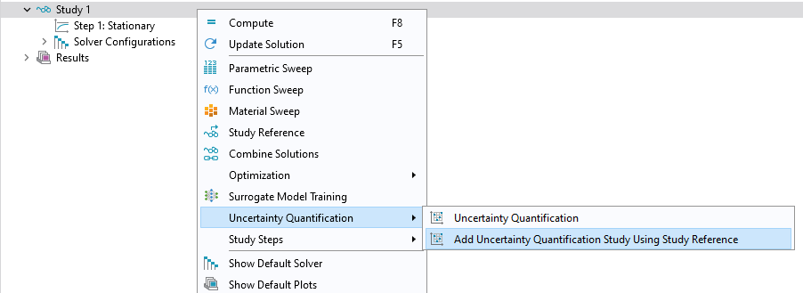A screenshot of part of the model tree with the Study 1 node selected and the menu of study types that can be added displayed, with the Uncertainty Quantification options expanded.

Adding the Uncertainty Quantification study referencing the static structural study.

The Uncertainty Quantification study gives the option to choose among five different UQ study types for screening, sensitivity analysis, uncertainty propagation, reliability analysis, and inverse UQ. The default UQ study type is Screening, MOAT, as shown in the figure below.

The Uncertainty Quantification study settings with UQ study type set to Screening, MOAT_._

The next step is to add the quantity of interest, which in this case is the misalignment angle with the variable name phi. This variable is added to the Quantities of Interest section in the Uncertainty Quantification study Settings window. However, since the Uncertainty Quantification study can reference several different components, we need to specify this variable as comp1.phi. (If there was a second component, comp2, there could also be a variable in that component with the name phi, which would be referred to as comp2.phi.) Instead of typing the name comp.phi, you can click the Expression field and press Ctrl+Space (code completion) to locate the variable in the tree, as shown in the figure below.

The Quantities of Interest specification in the Uncertainty Quantification study Settings window.

In the Input Parameters section, start by adding the first input parameter ts for the material thickness. Change the Distribution type to . Next, specify the Mean value to be ts and the Standard deviation value to be 0.01*ts. Change the CDF-Lower and CDF-Upper settings to Manual. For the Lower bound setting, enter 0.99*ts, and for the Upper bound setting, enter 1.01*ts, as shown in the figure below.

The material thickness added as an input parameter with a normally distributed variability.

These values assumes that the material thickness has a normal distribution due to manufacturing variability. The truncation defined by the bounds corresponds to the part that is rejected if the thickness is outside these limits (i.e., if it is too thin or too thick).

The normal distribution for the material thickness with the lower and upper bounds indicated. The truncated distribution is normalized so that the integrated area equals one.

Now, continue to enter the input parameters and distribution settings for the other input parameters according to the earlier table and figure below.

The input parameters for the screening analysis.

Run the Simulation

The study settings are now prepared for the screening analysis. To start the computation, right-click Study 2 and select Compute.

Once the computation is complete (which takes about 10 minutes, depending on the hardware), a MOAT scatter diagram is shown by default. The diagram shows the MOAT mean and standard deviation for each input parameter, as illustrated in the figure below.

The MOAT mean and MOAT standard deviation values for each input parameter.

In addition, a MOAT table shows the mean and standard deviation values, as shown below.

The MOAT table displaying the mean and standard deviation values.

Visualize and Analyze the Results

The diagram and the table provide insight into the influence of each input parameter on the misalignment angle. We observe that the side length (ls) and the cross-plate width (wp) are most likely the most influential parameters. The flange width (wf) also appears to have a significant effect, though to a lesser extent. However, the relative differences among the less influential input parameters are not pronounced enough to definitively determine which can be neglected.

The parameters fr1 and ts seem to have minimal impact, yet their MOAT mean values are still significantly greater than zero. This indicates that the screening does not conclusively identify negligible parameters. Therefore, a more detailed analysis is necessary to clearly differentiate between the parameters. This can be accomplished through the sensitivity analysis option offered as one of the UQ study types, which is demonstrated in the next part of this course. Note that the model with the completed screening analysis is available for download and will serve as the starting point for the sensitivity analysis conducted in the next part.